Aggregate Supply

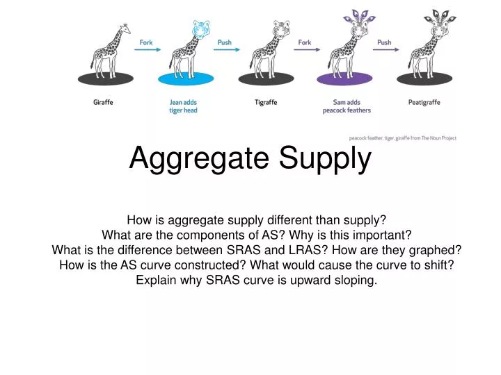
1. Aggregate Supply How is aggregate supply different than supply? What are the components of AS? Why is this important? What is the difference between SRAS and LRAS? How are they graphed? How is the AS curve constructed? What would cause the curve to shift? Explain why SRAS curve is upward sloping.

2. Aggregate Supply • Aggregate supply (AS) measures the volume of goods and services produced within the economy at a given price level • In other words: amount of real GDP that will be made available by sellers at various price levels when resource prices (i.e., wages) do not change • Represents the ability of an economy to deliver goods and services to meet demand • Nature of this relationship will differ between the long run and the short run • Short run aggregate supply (SRAS) shows total planned output when prices in the economy can change but the prices and productivity of all factor inputs e.g. wage rates and the state of technology are held constant. • In the short run, the SRAS curve is assumed to be upward sloping (i.e. it is responsive to a change in aggregate demand reflected in a change in the general price level) • Long run aggregate supply (LRAS):  LRAS shows total planned output when both prices and average wage rates can change – it is a measure of a country’s potential output and the concept is linked to the production possibility frontier • In the long run, the LRAS curve is assumed to be vertical (i.e. it does not change when the general price level changes)

3. Aggregate Supply Curve The aggregate supply curve shows the relationship between the aggregate price level and the quantity of aggregate output. Aggregate Supply looks different in the Long Run and the Short Run: In the Long Run, classical economists assume the economy operates at full employment (maximum output), independent of the price level. In the Short Run, businesses will increase supply if the price level increases.

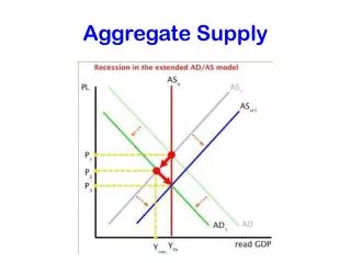
4. A change in the price level brought about by a shift in AD results in a movement along the short run AS curve. If AD rises, we see an expansion of SRAS; if demand falls we see a contraction of SRAS.

5. The Short-Run Aggregate Supply Curve

6. The SRAS is positively sloped because: • Auction markets • Prices are determined by demand and supply •  prices   profits   quantity supplied • Posted-price markets • Prices are set by producers and don’t often change • Firms respond to changes in demand by adjusting output instead of prices

7. Sticky Nominal Wages • The short-run aggregate supply curve is upward-sloping because nominal wages (dollar amount of the wage paid) are “sticky” in the short run: • Sticky: a variable is resistant to change • a higher aggregate price level leads to higher profits and increased aggregate output in the short run. • Market forces may reduce the real value of labor in an industry, but wages will tend to remain at previous levels in the short run. • Can be due to institutional factors: • price regulations • legal contractual commitments • labor unions • human stubbornness, human needs, or self-interest • Stickiness may apply in one direction. For example, a variable that is "sticky downward" will be reluctant to drop even if conditions dictate that it should. However, in the long run it will drop to the equilibrium level.

8. Movement vs. Shift • A change in aggregate price levels causes a movement along the SRAS curve. • However, a shift in SRAS is caused by changes in costs of production: • commodity prices (“non-labor resource prices”) • Expectations surrounding future inflation • Increase in import prices • nominal wages • business taxes (taxes on firms’ profits) • subsidies offered to businesses • supply shocks—events that have a sudden, strong impact on SRAS (weather, war…) • lead to changes in producers’ profits and shift the short-run aggregate supply curve

9. LEFT Increase in wages (if price level constant) Increase in price of non-labor resources Decrease in subsidies Unfavorable conditions (weather, conflict) RIGHT Wages decrease (price level constant) Decrease in price of non-labor resources Increase in subsidies Favorable conditions (weather) Shift in SRAS

10. The main cause of a shift in the supply curve is a change in business costs.

11. From the Short Run to the Long Run Leftward Shift of the Short-run Aggregate Supply Curve

12. From the Short Run to the Long Run Rightward Shift of the Short-run Aggregate Supply Curve

13. Long-Run Aggregate Supply (LRAS), part I “Seemingly small differences in growth rates can have a large impact over a period of many years. For example, if an economy grew by 2 per cent every year, it would double in size within 35 years; if it grew at 2½ per cent a year, it would double in size after 28 years - seven years earlier” Source: UK Treasury

14. LRAS • The long-run aggregate supply curve shows the relationship between the aggregate price level and the quantity of aggregate output supplied that would exist if all prices, including nominal wages, were fully flexible • LRAS is determined by the stock of a country’s resources and by the productivity of factor inputs (labour, land and capital). Changes in the technology also affect potential real national output. • In the long run, the ability of an economy to produce goods and services to meet demand is based on the state of production technology and the availability and quality of factor inputs. • A long run production function for a country is often written as follows: Y*t = (Lt, Kt, Mt) • Y* is a measure of potential output • t is the time period • L represents the quantity and ability of labor input available • Kt represents the available capital stock • Mt represents the availability of natural resources

15. A Range for Potential Output and the LAS Curve • The position of the long-run aggregate supply curve is determined by potential output– the amount of goods and services an economy can produce when both labor and capital are fully employed. • There are two models for LRAS: • Monetarist (new classical) • Keynesian

16. Key principles: Importance of the price mechanism in coordinating economic activities Competitive market equilibrium Economy is harmonious system that automatically tends towards full employment These are all points of contention in macroeconomics Shape of LRAS! Shown as vertical at potential GDP, or full employment level of GDP (YP) Means that in the long-run, a change in the price level does not result in any change in the quantity of real GDP produced Monetarist view of LRAS

17. Long-Run Aggregate Supply Curve

18. The economy is in long-run equilibrium when the AD curve and the SRAS curve intersect at any point on the LRAS curve p. 245, 248 in your home text p. 234, 237 Monetarist view of LRAS, cont.

19. LRAS is vertical line at full employment level of GDP (regardless of price level). WHY?! In the monetarist view, gaps are eliminated in the LR by flexibility in resource prices. This ensures that the LRAS curve will be vertical at the level of potential GDP. The economy then has a built-in tendency towards full-employment equilibrium. Long-Run Aggregate Supply Curve Real GDP = $6 trillion at every point on LRAS. Changes in AD can have an influence on real GDP only in the short run; in the long run, it only results in changing the price level, having no impact on real GDP (remains constant at level of potential output). So, increases in AD in long run are inflationary.

20. Resource Quantity: the quantity of the resources--labor, capital, land, and entrepreneurship--that the economy has available for production. include population growth, labor force participation, capital investment, and exploration. If the economy has more resources, more efficient: AS increases and LRAS curve shifts rightward. If the economy has fewer resources, less efficient: AS decreases and LRAS curve shifts leftward. Resource Quality: quality of resources, especially technology and education. labor, capital, land, and entrepreneurship Improved quality or reduction in unemployment increases AS, triggering a rightward shift of the LRAS curve Decline in quality or increase in unemployment decreases AS, generating a leftward shift of the LRAS curve Shifts in LRAS A shift in LRAS is caused by changes in any (ceteris paribus) factor other than the price level, such as natural rate of growth of output. LRAS curve can either shift rightward (increase in AS/real GDP/pos. econ. growth) or leftward (decrease in AS/real GDP/neg. econ. growth).

21. Any change in the economy that alters the natural rate of growth of output shifts LRAS. Improvements in productivity and efficiency or an increase in the stock of capital and labor resources cause the LRAS curve to shift out.

22. LAS1 Potential output Economic Growth Shifts the LRAS Curve Rightward • The LAScurve showsthe long- • run relationship between output • and the price level. LAS • The position of the LAS curve • depends on potential output – • the amount of goods and • services an economy can • produce when both capital and • labor are fully employed. Price Level • The LAS is vertical because • potential output is unaffected • by the price level. • Economic growth shifts the LRAS to the right. Real output

24. Econ growth=LRAS shifts right, signaling increase in potential output. However, SRAS curve will shift right because at any moment in time, economy is always producing on an SRAS curve. Any factor that shifts the LRAS curve must also shift SRAS curve. SRAS can be shifted temporarily from LRAS, such as unfavorable conditions. Changes in wages, or prices of key inputs (i.e., oil) may only affect SRAS curve. This applies only to changes that don’t have a lasting impact on GDP. How are SRAS and LRAS related?

25. TRY IT! • Rising investment shifts the aggregate demand curve to the right and at the same time shifts the long-run aggregate supply curve to the right by increasing the nation’s stock of physical and human capital. • Show this simultaneous shifting in the two curves with three graphs. • One graph should show growth in which the price level rises, • one graph should show growth in which the price level remains unchanged, • and another should show growth with the price level falling.

26. TRY IT! answers • Panel (a) shows AD shifting by more than LRAS; the price level will rise in the long run. • Panel (b) shows AD and LRAS shifting by equal amounts; the price level will remain unchanged in the long run. • Panel (c) shows LRAS shifting by more than AD; the price level falls in the long run.

27. The Following Slides are from your textbook.

28. Actual and Potential Output

29. When resources are over-utilized • (point C), factor prices may be bid • up and the SAS shifts up. • When resources are under-utilized • (point A), factor prices may decrease • and SAS shifts down. LAS Curve LAS • Estimating potential output is • inexact, so it is assumed to be the • middle of a range bounded by a • high level of potential output and a • low level of potential output. C • The relationship between • potential and actual output – where • the economy is on SAS – determines • shifts in SAS. B A SAS Price Level Underutilized resources Overutilized resources Real output Low-level potential output High-level potential output • When LAS = SAS (point B), there is • no pressure for prices to rise or fall.

30. Long-Run Macroeconomic Equilibrium LR equilibrium of $6 trillion in real GDP and price level of 100. Supply Creates Its Own Demand!

31. Short-Run Aggregate Supply Curve SRAS is relatively flat at low levels of output, and gradually approaches vertical. Beyond full employment GDP, expanding production is more expensive, so firms need large price increase output. At low levels of output, firms can easily expand output when prices rise.