Download
1 / 53
530 likes | 684 Views
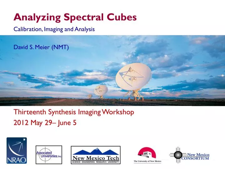
Analyzing Spectral Cubes. Calibration, Imaging and Analysis David S. Meier (NMT). Outline:. Why spectral line (multi-channel) observing? Not only for spectral lines, but there are many advantages for continuum experiments as well Calibration specifics

E N D
Analyzing Spectral Cubes Calibration, Imaging and Analysis David S. Meier (NMT)
Outline: • Why spectral line (multi-channel) observing? • Not only for spectral lines, but there are many advantages for continuum experiments as well • Calibration specifics • Bandpass, flagging, continuum subtraction • Imaging of spectral line data • Visualizing and analyzing cubes Thirteenth Synthesis Imaging Workshop
Radio Spectroscopy: • There is a vast array of spectral lines available, covering a wide range of science. van der Tak et al. (2009) • ALMA SV – Orion KL Courtesy A. Remijan • [CII] at a redshift of 7.1 Venemans et al. (2012) Thirteenth Synthesis Imaging Workshop
Introduction: Spectral line observers use many channels of width , over a total bandwidth . Why? • Science driven: science depends on frequency (spectroscopy) • Emission and absorption lines, and their Doppler shifts • Ideally we would like δv < 1 km/s over bandwidths of several GHz which requires thousand and thousands of channels • ALMA multiple lines: over 8 GHz, < 1km/s resolution~1 MHz Þ >8,000 channels • EVLA HI absorption: 1-1.4 GHz, < 1km/s resolution ~4 kHz Þ >100,000 channels Thirteenth Synthesis Imaging Workshop
CM linesBothMM lines Radio Spectroscopy: • Morphology and Kinematics • Atomic: HI • Molecular: CO, 13CO • Masers OH, H2O, CH3OH, SiO • Ionized: H186α – H50α • H42α – H22α • Dense Molecular Gas • HCN, HNC, HCO+, CS, NH3, HC3N • Chemistry • PDRs • Shocks & Outflows • Hot Cores • CH, CN, CCH, c-C3H2 • SiO, CH3OH, HNCO, H2S • CH3CN, ‘big floppy things’ • http://www.physics.nmt.edu/Department/homedirlinks/dmeier/echemprimer/ Thirteenth Synthesis Imaging Workshop
Introduction: • Science driven: science depends on frequency (pseudo-continuum). • Want maximum bandwidth for sensitivity [Thermal noise µ 1/sqrt(Dn)] • BUT achieving this sensitivity also requires high spectral resolution: • Source contains continuum emission with a significant spectral slope across Dn • Contaminating narrowband emission: • line emission from the source • RFI (radio frequency interference) • Changes in the instrument with frequency • Changes in the atmosphere with frequency • Technical reasons: science does not depend on frequency (pseudo-continuum) – particularly in the era of wide-band datasets • Changing primary beam with frequency • Limitations of bandwidth smearing Thirteenth Synthesis Imaging Workshop
2 Effects of Broad Bandwidth: • Changing Primary Beam (θPB = l/D) • θPB changes by l1/l2 • More important at longerwavelengths: • VLA 20 cm: 1.03 ; 2 cm: 1.003 • JVLA 20 cm: 2.0 ; 2 cm: 1.5 • ALMA 1mm: 1.03 Thirteenth Synthesis Imaging Workshop
11arcmin 18arcmin Effects of Broad Bandwidth: (u,v) for JVLA A-array, ratio 2.0 • Bandwidth Smearing (chromatic aberration) • Fringe spacing = l/B • Fringe spacings change by l1/l2 • u,v samples smeared radially • More important in larger configurations, and for lower frequencies • Huge effects for JVLA • Multi-frequency synthesis VLA-A 6cm: 1.01 Courtesy C. Chandler Thirteenth Synthesis Imaging Workshop
s s b X X X X n1 n1 n2 n2 n3 n3 n4 n4 Spectroscopy with Interferometers (Simple): • Simplest concept: filter banks • Output from correlator is r(u,v,n) • Very limited in its capabilities scientifically Thirteenth Synthesis Imaging Workshop
s s b X Spectroscopy with Interferometers (Lag): • Lag (XF) correlator: introduce extra lag t and measure correlation function for many (positive and negative) lags; FT to give spectrum SIRA 2 Thirteenth Synthesis Imaging Workshop
Spectroscopy with Interferometers (Lag): • In practice, measure a finite number of lags, at some fixed lag interval, Δτ • Total frequency bandwidth = 1/(2Δτ) • For N spectral channels have to measure 2N lags (positive and negative), from -NDt to +(N-1)Dt (zero lag included) • Spectral resolution dn = 1/(2NΔτ) (Nyquist) • Note: equal spacing in frequency, not velocity • Very flexible: can adjust N and Dt to suit your science Thirteenth Synthesis Imaging Workshop
Gibbs Ringing: • For spectroscopy in an XF correlator (EVLA) lags are introduced • The correlation function is measured for a large number of lags. • The FFT gives the spectrum. • We don't have an infinite amount of time, so we don't measure an infinite number of Fourier components. • A finite number or lags means a truncated lag spectrum, which corresponds to multiplying the true spectrum by a box function. • The spectral response is the FT of the box, which for an XF correlator is a sinc(x) function with nulls spaced by the channel separation: 22% sidelobes! "Ideal" spectrum Measured spectrum Amp Amp Frequency Frequency Thirteenth Synthesis Imaging Workshop
Gibbs Ringing (Cont.): Sampled: • Increase the number of lags, or channels. • Oscillations reduce to ~2% at channel 20, so discard affected channels. • Works for band-edges, but not for spectral features. • Smooth the data in frequency (i.e., taper the lag spectrum) • Usually Hanning smoothing is applied, reducing sidelobes to <3%. SIRA 2 Thirteenth Synthesis Imaging Workshop
JVLA Spectral Line Capabilities: • 2 x 1 GHz basebands • 16 tunable subbands per baseband (except avoid suckouts) with between 0.03125 – 128 MHz • Dual polarization: Up to 2000 channels per subband (up to 16,384 per baseband) • But data rate limitations 2 x 1 GHz Up to 2000 Thirteenth Synthesis Imaging Workshop
ALMA Spectral Line Capabilities: • Summary (Cycle 0): • Band 3,7 (6): 2 x 4(5) GHz sidebands, separated by 8 (10) GHz • 4 x 2 GHz basebands, with 0,2,4 distributed per sideband • 1 Spectral Windows per baseband, for a total of up to 4 • For dual polarization, bandwidths of each spectral window range from 0.0586 – 2 GHz • For dual polarization spectral resolution ranges from 0.0306 MHz – 0.976 MHz • Single polarization: you can get ~7.5 GHz simultaneously at ≤1.5 km/s Thirteenth Synthesis Imaging Workshop
Calibration: • Data editing and calibration is not fundamentally different from continuum observations, but a few additional items to consider: • Bandpass calibration • Presence of RFI (data flagging) • Doppler corrections Thirteenth Synthesis Imaging Workshop
Calibration - Bandpass: • We need the total response of the instrument to determine the true visibilities from the observed visibilities: obsVij(t,ν) = Gij(t,ν) Vij(t,ν) • The bandpass shape is a function of frequency, and is mostly due to electronics of individual antennas. • Atmosphere • Front end system • Cables • Inacurate clocks and antenna positions • Gibbs Phenomena • But typically not standing waves G/T @ 20cm Tsys @ 7mm JVLA Thirteenth Synthesis Imaging Workshop
Calibration - Bandpass (cont.): • Usually varies slowly with time, so we can break the complex gain Gij(t) into a fast varying frequency independent part, G’ij(t) and a slowly varying frequency dependent part, Bij(t,ν). Gij(t,ν) = G’ij(t) Bij(t,ν) • The demands on Bij(t) are different from those of G’ij(t,ν). • G’ij(t): point source, near science target • Bij(t,ν): very bright source, no spectral structure, does not need to be a point source (though preferable). • Observe a bright calibrator with the above properties at least once during an observation • Sometimes a noise source is used to BP, especially at high frequencies and when channels are very narrow • Still observe a BP calibrator • Bij(t,ν) can often be solved on an antenna basis: Bij(t,ν) = bi(t,ν)bj*(t,ν) • Computationally less expensive • Solutions can be found for antennas even with missing baselines Thirteenth Synthesis Imaging Workshop
Calibration - Bandpass (Issues): • Important to be able to detect and analyze spectral features: • Frequency dependent phase errors can lead to spatial offsets between spectral features, imitating Doppler motions. • Rule of thumb: θ/θB≅Δϕ/360o • Frequency dependent amplitude errors can imitate changes in line structures. • Need to spend enough time on the BP calibrator so that SNRBPcal >> SNRtarget. • Rule of thumb: tBPcal > 9(Starget /SBPcal)2 ttarget • When observing faint lines superimposed on bright continuum more stringent bandpass calibration is needed. • SNR on continuum limits the SNR achieved for the line • For pseudo-continuum, the dynamic range of final image is limited by the bandpass quality. Thirteenth Synthesis Imaging Workshop
Calibration - Bandpass: • Solutions should look comparable for all antennas. • Mean amplitude ~1 across useable portion of the band. • No sharp variations in amplitude and phase; variations are not dominated by noise. Not good, line feature Too weak Good Thirteenth Synthesis Imaging Workshop
Calibration - Bandpass: • Always check BP solutions: apply to a continuum source and use cross-correlation spectrum to check: • That phases are flat • That amplitudes are constant across band (continuum) • Absolute fluxes are reasonable • That the noise is not increased by applying the BP Before bandpass calibration After bandpass calibration Courtesy L. Matthews Thirteenth Synthesis Imaging Workshop
Calibration: • Data editing and calibration is not fundamentally different from continuum observations, but a few additional items to consider: • Bandpass calibration • Presence of RFI (data flagging) • Doppler corrections • Correlator setup Thirteenth Synthesis Imaging Workshop
Flagging Spectral Line Data (RFI): • Primarily a low frequency problem (for now) • Avoid known RFI if possible, e.g. by constraining your bandwidth (if you can) • Use RFI plots posted online for JVLA & VLBA RFI at the JVLA L-Band RFI at the JVLA S-Band Thirteenth Synthesis Imaging Workshop
Flagging Spectral Line Data: • Start with identifying problems affecting all channels, but using a frequency averaged 'channel 0' data set. • Has better signal-to-noise ratio (SNR) • Copy flag table to the line data • Continue checking the line data for narrow-band RFI that may not show up in averaged data. • Channel by channel is very impractical, instead identify features by using cross- and total power spectra (POSSM) • Avoid extensive channel by channel editing because it introduces variable (u,v) coverage and noise properties between channels (AIPS: SPFLG, CASA:MSVIEW) time channel Thirteenth Synthesis Imaging Workshop
Calibration: • Data editing and calibration is not fundamentally different from continuum observations, but a few additional items to consider: • Bandpass calibration • Presence of RFI (data flagging) • Doppler corrections Thirteenth Synthesis Imaging Workshop
Doppler Tracking: • Observing from the surface of the Earth, our velocity with respect to astronomical sources is not constant in time or direction. • Doppler tracking can be applied in real time to track a spectral line in a given reference frame, and for a given velocity definition: • Vrad = c (νrest –νobs)/νrest(approximations to relativistic formulas) • Vopt = c (νrest –νobs)/νobs = cz • Differences become large as redshift increases • For the Vopt definition, constant frequency increment channels do not correspond to constant velocities increment channels Thirteenth Synthesis Imaging Workshop
Doppler Tracking: • Note that the bandpass shape is really a function of frequency, not velocity! • Applying Doppler tracking will introduce a time-dependent and position dependent frequency shift. • If differences large, apply corrections during post-processing instead. • With wider bandwidths are now common (JVLA, SMA, ALMA) online Doppler setting is done but not tracking (tracking only correct for a single frequency). • Doppler tracking is done in post-processing (AIPS/CASA: CVEL/CLEAN) • Want well resolved lines (>4 channels across line) for good correction Amp Amp Channel Channel Thirteenth Synthesis Imaging Workshop
Velocity Reference Frames: Start with the topocentric frame, the successively transform to other frames. Transformations standardized by IAU. Thirteenth Synthesis Imaging Workshop
Imaging: • We have edited the data, and performed bandpass calibration. Also, we have done Doppler corrections if necessary. • Before imaging a few things can be done to improve the quality of your spectral line data • Image the continuum in the source, and perform a self-calibration. Apply to the line data: • Get good positions of line features relative to continuum • Can also use a bright spectral feature, like a maser • For line analysis we want to remove the continuum Thirteenth Synthesis Imaging Workshop
Continuum Subtraction: • Spectral line data often contains continuum emission, either from the target or from nearby sources in the field of view. • This emission complicates the detection and analysis of lines • Easier to compare the line emission between channels with continuum removed. • Use channels with no line features to model the continuum • Subtract this continuum model from all channels • Always bandpass calibrate before continuum subtracting • Deconvolution is non-linear: can give different results for different channels since u,v - coverage and noise differs • results usually better if line is deconvolved separately • Continuum subtraction changes the noise properties of the channels Roelfsma 1989 Spectral line cube with two continuum sources (structure independent of frequency) and one spectral line source. Thirteenth Synthesis Imaging Workshop
Continuum Subtraction (UVLIN): • Advantages: • Fast, easy, robust • Corrects for spectral index across spectrum • Can do flagging automatically (based on residuals on baselines) • Can produce a continuum data set • Restrictions: • Fitted channels should be line free (a visibility contains emission from all spatial scales) • Only works well over small field of view • << B / tot • A low order polynomial is fit to a group of line free channels in each visibility spectrum, the polynomial is then subtracted from whole spectrum. SIRA 2 • For a source at distance l from phase center observed on baseline b: Thirteenth Synthesis Imaging Workshop
Continuum Subtraction (IMLIN): • Fit and subtract a low order polynomial fit to the line free part of the spectrum measured at each spatial pixel in cube. • Advantages: • Fast, easy, robust to spectral index variations • Better at removing point sources far away from phase center (Cornwell et al.1992). • Can be used with few line free channels. • Restrictions: • Can't flag data since it works in the image plane. • Line and continuum must be simultaneously deconvolved. Thirteenth Synthesis Imaging Workshop
Continuum Subtraction (UVSUB): • A visibility + imaging based method • Deconvolve the line-free channels to make a ‘model’ of the continuum • Fourier transform and subtract from the visibilities • Advantages: • Accounts for chromatic aberration • Channel-based flagging possible • Can be effective at removing extended continuum over large fields of view • Restrictions: • Computationally expensive • Errors in the ‘model’ (e.g. deconvolution errors) will introduce systematic errors in the line data Thirteenth Synthesis Imaging Workshop
Continuum Subtraction: • Again check results: Look at spectrum with POSSM, and later (after imaging) check with ISPEC: no continuum level, and a flat baseline. Courtesy L. Matthews Thirteenth Synthesis Imaging Workshop
Deconvolution (Spectral Line): • HC3N – IRC 10216 • CLEANing: • Remove sidelobes that would obscure faint emission (masers, significant extended emission) • Interpolate to zero spacings to estimate flux • Deconvolution poses special challenges • Spectral line datasets are inherently detailed comparisons of the morphology of many maps • Emission structure can change radically from channel to channel • Large data volumes / computationally expensive EVLA spectral line tutorial Thirteenth Synthesis Imaging Workshop
Deconvolution (Spectral Line): • Spatial distribution of emission changes from channel to channel: • Try to keep channel-to-channel deconvolution as similar as possible (same restoring beam, same CLEANing depth, etc.) • May have to change cleaning boxes from channel to channel • Want both: • Sensitivity for faint features and full extent of emission • High spectral & spatial resolution for kinematics • Averaging channels will improve sensitivity but may limit spectral resolution • Choice of weighting function will affect sensitivity and spatial resolution • Robust weighting with -1<R <1 is often a good compromise • Interferometer response is sensitive to velocity structure of object • Response to continuum and spectral line is not necessarily the same Thirteenth Synthesis Imaging Workshop
Smoothing (Spectral Line): • In frequency: • Smoothing in frequency can improve S/N in a line if the smoothing kernel matches the line width ("matched filter"). • And reduce your data size (especially if you oversampled) • Smoothing doesn’t propagate noise in a simple way • Example: data are Hanning smoothed to diminish Gibbs ringing • Spectral resolution will be reduced from 1.2 to 2.0 • Noise equivalent bandwidth is now 2.67 • Adjacent channels become correlated: ~16% between channels i and i+1; ~4% between channels i and i+2. • Spatially: • Smoothing data spatially (through convolution in the image plane or tapering in the u-v domain) can help to emphasize faint, extended emission. • This only works for extended emission. • Cannot recover flux you didn’t sample Thirteenth Synthesis Imaging Workshop
Visualizing Spectral data: • Imaging will create a spectral line cube, which is 3-dimensional: RA, Dec and Velocity. • Movies: • HI - NGC 3741 Courtesy J. Ott (VLA-ANGST) Thirteenth Synthesis Imaging Workshop
Visualizing Spectral data: • HI – NGC 3741 • 3rd axis not the same as the first two • Imaging will create a spectral line cube, which is 3-dimensional: RA, Dec and Velocity. • 3-D Rendering: • Displayed with the ‘xray’ program in the visualization package ‘Karma’ (http://www.atnf.csiro.au/computing/software/karma/) Thirteenth Synthesis Imaging Workshop
Visualizing Spectral data: • 13CO(1-0) – Maffei 2 • Imaging will create a spectral line cube, which is 3-dimensional: RA, Dec and Velocity. • 3-D Rendering: • Displayed with the ‘xray’ program in the visualization package ‘Karma’ (http://www.atnf.csiro.au/computing/software/karma/) Meier et al. (2008) Thirteenth Synthesis Imaging Workshop
HC3N – IRC 10216 Channel Maps: • Channel maps show how the spatial distribution of the line feature changes with frequency/velocity. CASA spectral line tutorial Thirteenth Synthesis Imaging Workshop
+Vcir sin i cos +Vcir sin i -Vcir sin i -Vcir sin i cos Inclined Disks: ‘Butterfly Pattern’:
CO(1-0) – IRC 10216 Fong et al. (2003) Spherical Shells: Thirteenth Synthesis Imaging Workshop
Visualizing Spectral data: • Imaging will create a spectral line cube, which is 3-dimensional: RA, Dec and Velocity. • With the cube, we usually visualize the information by making 1-D or 2-D projections: • Moment maps (integration along the velocity axis) • Line profiles (1-D slices along velocity axis) • Channel maps (2-D slices along velocity axis) • Position-velocity plots (slices along spatial dimension) • Renzograms (superposed contours of different channels) Thirteenth Synthesis Imaging Workshop
Moment Maps: • You might want to derive parameters such as integrated line intensity, centroid velocity of components and line widths - all as functions of positions. Estimate using the moments of the line profile: Courtesy L. Matthews Moment 0 Moment 1 Moment 2 (Total Intensity) (Velocity Field) (Velocity Dispersion) Thirteenth Synthesis Imaging Workshop
Moment Map Issues: • Moments sensitive to noise so clipping is required • Higher order moments depend on lower ones so progressively noisier. Straight sum of all channels containing line emission Summed after clipping below 1 Summed after clipping below 2 Clipping below 1 , but based on masking with a cube smoothed x2 spatially and spectrally Courtesy L. Matthews Thirteenth Synthesis Imaging Workshop
Moment Map Issues (cont.): • Hard to interpret correctly: • Non-monotomic emission/absorption or velocity patterns lead to misleading moment maps • Biased towards regions of high intensity. • Complicated error estimates: number or channels with real emission used in moment computation will greatly change across the image. • Use as guide for investigating features, or to compare with other . Moment 2 Moment 0 Meier et al. (2008) Thirteenth Synthesis Imaging Workshop
Position-Velocity diagrams: Courtesy L. Matthews • PV-diagrams show, for example, the line emission velocity as a function of radius. • Here along a line through the dynamical center of the galaxy Velocity profile Meier et al. (2008) Distance along slice Thirteenth Synthesis Imaging Workshop
Hatchell et al. (2007) Renzograms: • Contour selected planes (usually redshifted, systemic and blueshifted), and superpose onto one plane • Often done when velocity structure is very simple or very complex Zuckerman et al. (2008) Thirteenth Synthesis Imaging Workshop
3 3 4 10 1 5 11 2 6 12 7 4 13 8 9 10 5 1 11 6 2 12 7 13 8 9 Line profiles (spectra): • Line profiles show changes in line shape, width and depth as a function of position. • AIPS task ISPEC Courtesy Y. Pihlstrom Thirteenth Synthesis Imaging Workshop