Download
1 / 17
350 likes | 1.13k Views
Phase Equilibria. X(phase 1) X(phase 2) At equilibrium, D G = 0 so µ(phase 1) = µ(phase 2) For boiling: K = a(g)/a(l) Gases fairly ideal so a(g) = P(atm) Activity of liquid set to 1: a(l) = 1 Equilibrium constant K = P P 1 , P 2 are equilibium vapor pressures at T 1 and T 2

E N D
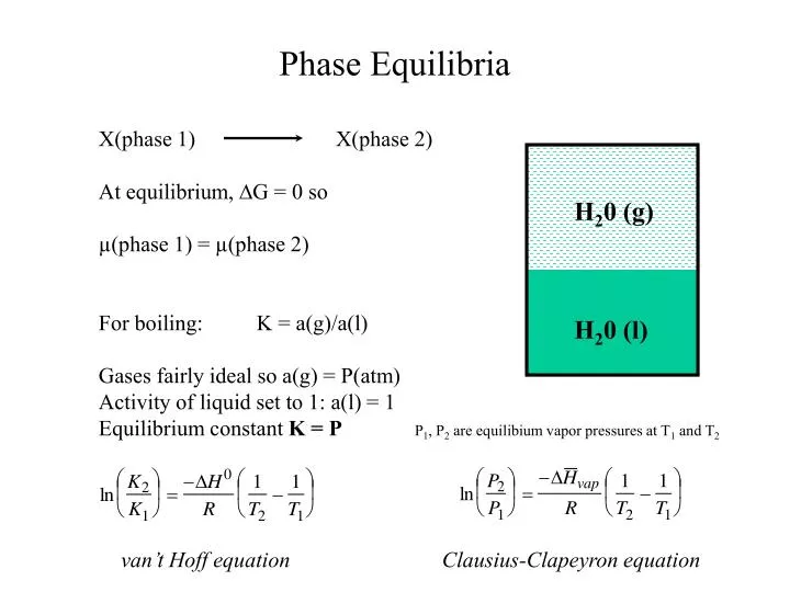
Phase Equilibria X(phase 1) X(phase 2) At equilibrium, DG = 0 so µ(phase 1) = µ(phase 2) For boiling: K = a(g)/a(l) Gases fairly ideal so a(g) = P(atm) Activity of liquid set to 1: a(l) = 1 Equilibrium constant K = PP1, P2 are equilibium vapor pressures at T1 and T2 van’t Hoff equation Clausius-Clapeyron equation H20 (g) H20 (l)
liquid water solid ice DHvap ln P(atm) DHsub water vapor 1/T Vapor Pressure DH can be determined from measurements of vapor pressure at multiple temperatures. From Clausius-Clapeyron equation we see that -DH/R is the slope lnP vs 1/T. Example Problem: At what pressure (or altitude) does water boil at body temperature? Get the pressure first, then estimate the altitude. DH not completely independent of T
Pressure Dependence of Melting Temperature For reversible processes: Heat of fusion is always positive. Volume of fusion is usually positive, but it is negative for water.
Mixtures: vapor pressure For each component, i, in the mixture: µi(phase 1) = µi (phase 2) Vapor pressure µA(solution) = µA(g, PA) Letting µ*A and P*A refer to the pure solvent, µA(g, PA) = µ*A(g, P*A) + RTln(PA/ P*A) At equilibrium, µA(g, PA) = µA(solution) so, µA(solution) = µ*A(pure solvent) = RTln(PA/ P*A) = RTln(aA) Solvent activity can be determined by measuring the vapor pressure. aA = PA/ P*A H2O (g) O2(g) H2O (l) O2(aq)
Mixtures: Raoult’s law Solvent activity is related to the vapor pressure aA = PA/ P*A (PA = vapor pressure solution) (P*A = vapor pressure pure solvent) Activity of the solvent can be expressed as aA = gAXA (where XA is the mole fraction) Then for ideal solutions, gA = 1 and PA = XA P*A This is Raoult’s law for ideal solutions. Applies to the solvent. H2O (g) O2(g) H2O (l) O2(aq)
Mixtures: Henry’s law Focus on the solute (e.g. O2) O2(g) O2(aq) Keq = PO2 = kO2XO2 PO2 = vapor pressure of O2 XO2 = mole fraction of O2 in liquid kO2 = Henry’s law constant (measured experimentally; tabulated TSWP p. 194) Gas solubility is directly proportional to the gas partial pressure. Consider the relation between a faming bottle of champagne and the Bends. H2O (g) O2(g) H2O (l) O2(aq) Facts about O2: XO2(air) = 0.2 XO2(water) = 4.7 x 10⁻⁶ [O2](water) = 0.03[O2](air) (mol/liter)
Example H2O (g) O2(g),N2(g) Ar(g) Calculate the vapor pressure of water in equilibrium with air at 1atm, 25 °C. Calculate the total mole fraction of air dissolved in the water first. From Raoult’s law we have, The vapor-pressure lowering of water due to air solubility is negligible. The 3% of water in air (humidity at equilibrium) is not negligible, however. H2O (l) O2(aq), N2(aq) Ar(aq) Air data O2(g) 20.95% N2(g) 78.08% Ar(g) 0.93% Henry’s constants kO2 = 4.3 x 10² kN2 = 8.5 x 10² kAr = 3.9 x 10² Water data P*H2O = 0.031 atm (25 °C)
Multiple Phases At equilibrium, chemical potential for each component is the same in all three phases. Direct contact is not needed. Immiscible liquids, such as decane and water, can form phases. Semipermeable barriers can also be used to create effectively different phases - cell membranes (lipid bilayers) - dialysis membranes (nanoporous materials) Even molecular binding can be thought of in this way - bound vs free ligand (O2, hemoglobin) H2O (g) O2(g), N2(g) Ar(g), C7H16(g) H2O (l) O2(aq), N2(aq) Ar(aq), C7H16(aq) H2O (C7H16) O2(C7H16), N2(C7H16) Ar(C7H16), C7H16(l)
Multiple Phases: equilibrium without contact µA(s) = µA(aq) = µA(C7H16) The solute in water is in equilibrium with its counterpart in heptane even though they are not in contact. The activity of the solute in each saturated (equilibrium) solution can be used to calculate the standard chemical potential for the solute in that solvent relative to the solid. This provides a basis for comparison and we can determine Dµ0A = µ0A (C7H16) - µ0A (aq) the change in chemical potential when the solute is transferred from water to heptane. H2O (l) Solute (aq) Solid C10H22(l) Solute (C7H16) Solid
Example: Hydrophobicity • For the series of fatty acids CnH2n+1COOH • With n ≥ 5, generally more soluble in organic solvent than water • For palmitic acid (C15H31COOH) Dµ0A = µ0A (C7H16) - µ0A (aq) = -38 kJ/mol • For the series 8 ≤ n ≤ 22 Dµ0A = µ0A (C7H16) - µ0A (aq) = 17.82 - 3.45n kJ/mol • The hydrophobic core of a lipid membrane is a similar environment to organic solvents such as heptane. • Measurements of Dµ0A such as above relate to how molecules partition into cell membranes. See TSWP p. 208 for experimental data COOH (Hydrophilic) CH2 groups Hydrophobic
Side chain Index Side chain Index Isoleucine 4.5 Valine 4.2 Leucine 3.8 Phenylalanine 2.8 Cystein 2.5 Methionine 1.9 Alanine 1.8 Glycine -0.4 Threonine -0.7 Serine -0.8 Tryptophan -0.9 Tyrosine -1.3 Proline -1.6 Histidine -3.2 Glutamic Acid -3.5 Glutamine -3.5 Aspartic Acid -3.5 Asparigine -3.5 Lysine -3.9 Arginine -4.5 Hydropathy Index • Hydropathy index is the relative hydrophobicity-hydrophilicity of the side-chain groups in proteins at neutral pH. • Various methods of ranking exist • Negative values characterize hydrophilic groups • Positive values characterize hydrophobic groups • This has been used as a starting point to understand basic thermodynamics of protein folding.
Transfer between same solvents For transfer of a solute molecule between different solutions in the same solvent: DµA = µA(solution 2) - µA(solution 1) = RT ln(aA(solution 2)/aA(solution 1)) If the activity coefficients are the same in the two solutions DµA = RT ln(cA(solution 2)/cA(solution 1)) This is the free energy that drives diffusion and is the free energy of mixing.
Transfer of charged molecules Electric field does work on ion as it passes between solutions. DµA = µA(solution 2) - µA(solution 1) + ZFV V = (f2 - f1) potential difference in volts between the two solutions. F = Faraday = 96,485 (eV-1) = charge of mole of electrons. Z = charge of the ion (e.g. ±1) Note: this is true for any f(x). Convenient to write: µA,tot = µA + ZFf [Na+](1) [Cl-](1) f1 [Na+](2) [Cl-](2) f2 f1 Electrical Potential (f) f2 Position (x)
Equilibrium Dialysis Example At equilibrium: O2(out) = O2(in, aq) [Mb·O2]/[Mb][O2(aq)] = Keq If we are able to asses the total ligand concentration in the dialysis bag: [O2(aq)] + [Mb·O2] = [O2 (in, total)] Then [Mb·O2] = [O2 (in, total)] - [O2(aq)] (these are measurable) Can compute Keq. If we have direct a probe for Mb·O2, then we don’t need the dialysis, can read of concentrations and compute Keq. Dialysis can also be used to exchange solution (eg. change [salt]) H2O (l) O2(aq), N2(aq) etc. H2O (l) O2(aq), N2(aq) Mb(aq), Mb·O2(aq) Semipermeable membrane (cellulose): allows water and dissolved small solutes to pass, blocks passage of large proteins such as myoglobin (Mb)
Scatchard Equation General version: M + A M·A Keq = [M·A]/([M][A]) Simplify by introducing n, the average number of ligand molecules (A) bound to the macromolecule (M) at equilibrium: Scatchard plot NKeq Slope = -Keq n/[A] Scatchard equation N independent binding sites per macromolecule. For one ligand binding site per macromolecule n N
Cooperative Binding For a macromolecule with multiple binding sites, binding to one site can influence binding properties of other sites. Failure of data plotted in a Scatchard plot to give a straight line indicates cooperative or anticooperative binding among binding sites. Cooperative = binding of second ligand is made easier Anticooperative = binding of second ligand is made more difficult Hemoglobin is a favorite example of a protein with cooperative binding behavior. • Binds up to 4 O2 • Cooperative: most O2 released in tissue while binding O2 maximally in the lungs • Binding curve shows characteristic sigmoidal shape 1 Myoglobin Hemoglobin f p50 = 1.5 Torr p50 = 16.6 Torr f = fraction of sites bound 0 PO2(Torr) 0 40
Hill Plot Scatchard equation (non-cooperative binding) For cooperative binding. n = Hill coefficient K = a constant, not the Keq for a single ligand Slope of each line give the Hill cooperativity coefficient. Slope = 1 no cooperativity Slope = N maximum (all-or-nothing) cooperativity See Example 5.4 (TSWP p. 204 - 207) for a detailed study of Hemoglobin 1.5 Myoglobin n = 1.0 log[f /(1-f)] Hemoglobin n = 2.8 -1.5 -0.5 +2 log[P02] (Torr)