Download

1 / 54
540 likes | 542 Views
ICL Landslide Teaching Too l s. PPT-tool 1.064-1.3 ( 1 ). Probabilistic landslide hazard, North Island, New Zealand. G.D. Dellow. GNS Science (Lower Hutt, New Zealand) e-mail: g.dellow@gns.cri.nz. ICL Landslide Teaching Too l s. PPT-tool 1.064-1.3 ( 2 ). Outline. Definitions

E N D
ICL Landslide Teaching Tools PPT-tool 1.064-1.3 (1) Probabilistic landslide hazard, North Island, New Zealand G.D. Dellow GNS Science (Lower Hutt, New Zealand) e-mail: g.dellow@gns.cri.nz
ICL Landslide Teaching Tools PPT-tool 1.064-1.3 (2) Outline • Definitions • “All landslides” probabilistic landslide hazard model • Probabilistic hazard model for rainstorm-induced landslides
ICL Landslide Teaching Tools PPT-tool 1.064-1.3 (3) Definitions • Hazard and risk are terms often used inter-changeably. Both terms are derived from the same source – originally a card game, Hazard in English and Risk in French. • In scientific terms they each have a very specific meaning. Although hazard has dual use.
ICL Landslide Teaching Tools PPT-tool 1.064-1.3 (4) Definitions • Hazard “event” – in the context of this course a physical landslide. • Hazard “probability” – the likelihood of a landslide event. • (Some literature refers to this as “risk” and hence the confusion that can sometimes arise) • Risk – a product of the hazard and the consequences of a hazard event • What is the probability of incurring a specified loss within a specified time through the occurrence of a hazard event?
ICL Landslide Teaching Tools PPT-tool 1.064-1.3 (5) Definitions • Hazard = Probability of a landslide occurring • “All landslide” context (i.e. all landslides) • A probabilistic landslide hazard model for the North Island of New Zealand is presented as an example • Probability can also be driven by the probability of the triggering event (e.g. rainstorm or earthquake). • A rainstorm-induced probabilistic landslide hazard model is presented as an example
ICL Landslide Teaching Tools PPT-tool 1.064-1.3 (6) Probabilistic Landslide Hazard Model for the North Island • Considers all landslides • Combines all landslide types • Data includes both pre-existing landslides and first-time landslides • All movement rates considered
ICL Landslide Teaching Tools PPT-tool 1.064-1.3 (7) Probabilistic Landslide Hazard Model for the North Island The process: • The landslide data sets are described • Terrains are selected to reflect common geology, topography and landslide density • Magnitude-frequency curves are determined from the data sets and calibrated with respect to time for a uniform area • Relative landslide hazard maps are derived for various return periods and landslide sizes
ICL Landslide Teaching Tools PPT-tool 1.064-1.3 (8) The New Zealand Landslide Database • Inventory: holds geographic (area) locations of landslides • (for the North Island there are 5773 mapped landslides) • Catalogue: includes time of movement as well as geographic location • August 1996 – present (continuous record) • Pre-historic to July 1996 (incomplete) • 150-yr earthquake induced landslide record
ICL Landslide Teaching Tools PPT-tool 1.064-1.3 (9) The Landslide Inventory Prepared from air photo interpretation Transferred to topographic maps Then digitised
ICL Landslide Teaching Tools PPT-tool 1.064-1.3 (10) Inventory data magnitude/frequency curve • Data (5773 landslides) • Probability density distribution by landslide area
ICL Landslide Teaching Tools PPT-tool 1.064-1.3 (11) Inventory data magnitude/frequency curve • Data (5773 landslides) • Curve fitting • Binary bins (provides uniform fit across a logarithmic scale)
ICL Landslide Teaching Tools PPT-tool 1.064-1.3 (12) Inventory data magnitude/frequency curve • Data (5773 landslides) • Curve fitting • Binary bins • Inverse-gamma • Double pareto • Β=2.52±0.03 using binary bins (comparable to magnitude/frequency relationships given for landslides in international literature)
ICL Landslide Teaching Tools PPT-tool 1.064-1.3 (13) Catalogue data magnitude/frequency curve • Data (53 landslides) • The Catalogue data contains information about time of occurrence
ICL Landslide Teaching Tools PPT-tool 1.064-1.3 (14) Catalogue data magnitude/frequency curve • Data (53 landslides) • Curve fitting • Binary bins • 2.37±0.07 (c.f inventory at 2.52±0.03 - equivalent at 95% confidence) • Key assumption is that magnitude/frequency relationships for inventory and catalogue are equivalent (not significantly different)
ICL Landslide Teaching Tools PPT-tool 1.064-1.3 (15) 11 Terrains based on • Geology • Topography • Landslide density
ICL Landslide Teaching Tools PPT-tool 1.064-1.3 (16) Examples – Terrain I • Orongorongo River Valley, Wellington, 2005: intense rainfall trigger
ICL Landslide Teaching Tools PPT-tool 1.064-1.3 (17) Examples – Terrain I • Hutt River, Wellington, 2004: intense rainfall trigger
ICL Landslide Teaching Tools PPT-tool 1.064-1.3 (18) Power law curves for individual terrains • Terrain I • Indurated Mesozoic sandstones and siltstones • Number of landslides • 964 • Slope of the magnitude/frequency curve • 2.64 ± 0.05 • Percentage of total landslide population • 16.7%
ICL Landslide Teaching Tools PPT-tool 1.064-1.3 (19) Examples – Terrain III • Waingake, East Cape, 2002: intense rainfall trigger
ICL Landslide Teaching Tools PPT-tool 1.064-1.3 (20) Examples – Terrain IVb • Tangitu Road, King Country, 1998: prolonged rainfall trigger
ICL Landslide Teaching Tools PPT-tool 1.064-1.3 (21) Examples – Terrain IVa • Wangaehu Valley, Wanganui: inventory example
ICL Landslide Teaching Tools PPT-tool 1.064-1.3 (22) Power law curves for individual terrains • Terrain III • Tertiary sandstones, siltstones and limestones • Number of landslides • 1583 • Slope of the magnitude/frequency curve • 2.38 ± 0.12 • Percentage of total landslide population • 27.1%
ICL Landslide Teaching Tools PPT-tool 1.064-1.3 (23) Examples – Terrain VI Oaonui Stream, Mt Taranaki, 1998: intense rainfall triggered debris flow
ICL Landslide Teaching Tools PPT-tool 1.064-1.3 (24) Power law curves for individual terrains • Terrain VI • Active andesitic volcanoes • Number of landslides • 116 • Slope of the magnitude/frequency curve • 1.30 ± 0.07 • Percentage of total landslide population • 2.0%
ICL Landslide Teaching Tools PPT-tool 1.064-1.3 (25) Hazard curvesAbsolute hazard • Terrain hazard curve • Take the number of landslides >1000 m2 in 7 years for each terrain • Derive an annual rate for each terrain (point) • Plot the terrain magnitude/frequency relationship (slope of line) through the annual rate point
ICL Landslide Teaching Tools PPT-tool 1.064-1.3 (26) Absolute hazard map • Size of largest landslide expected on an annual basis High: 1000-10,000 m2 Moderate: 100-1000 m2 Low: 0-100 m2
ICL Landslide Teaching Tools PPT-tool 1.064-1.3 (27) Hazard curvesRelative hazard • Annual rate • Normalise for area (10,000 km2) • Plot
ICL Landslide Teaching Tools PPT-tool 1.064-1.3 (28) Relative Hazard Maps • Largest landslide expected in 1year High: 1000-10,000 m2 Moderate: 100-1000 m2
ICL Landslide Teaching Tools PPT-tool 1.064-1.3 (29) Relative Hazard Maps • Largest landslide expected in 100 years High: 109-1010 m2 Moderate: 10,000-100,000 m2 Low: 1000-10,000 m2
ICL Landslide Teaching Tools PPT-tool 1.064-1.3 (30) Relative Hazard Maps • Return period for landslides with an area greater than 1000 m2 High: 0-1 years Moderate: 1-10 years Low: 10-100 years
ICL Landslide Teaching Tools PPT-tool 1.064-1.3 (31) Relative Hazard Maps • Return period for landslides with an area greater than 1,000,000 m2 High: 1-10 years Moderate: 1000-10,000 years Low: 10,000-100,000 years Very low: 100,000-1,000,000 years
ICL Landslide Teaching Tools PPT-tool 1.064-1.3 (32) Results • Landslide area distributions for the North Island, New Zealand have a power-law magnitude/frequency relationship. • Selecting areas delineated on the basis of similar geology, topography and landslide density yields a range of magnitude/frequency relationships for landslide area distributions. • Landslide magnitude/frequency curves can be temporally calibrated using historical landslide data. • Five distinct landslide magnitude/frequency curves are recognised in the North Island, New Zealand.
ICL Landslide Teaching Tools PPT-tool 1.064-1.3 (33) Rainstorm-induced probabilistic landslide hazard model • Trigger is limited to rainstorm-induced landslides • Probability is determined by the probability of 24-hr rainfall occurring • Only considers first-time landslides • Only considers fast landslides
ICL Landslide Teaching Tools PPT-tool 1.064-1.3 (34) Premise • There is a relationship between rainfall intensity and landslide density • i.e. the greater the amount of rainfall, the greater the density of landslides • However landslide occurrence is also controlled by other factors such as slope angle, geology, vegetation
ICL Landslide Teaching Tools PPT-tool 1.064-1.3 (35) Premise • The basic premise of the model is that it: • takes rainfall data, • processes the data to produce a landslide forecast and then • distributes landslides in the landscape, either on a scenario basis or a probabilistic basis. • This model therefore has three components: • INPUT DATA • LANDSLIDE FORECAST MODEL • OUTPUT DATA
ICL Landslide Teaching Tools PPT-tool 1.064-1.3 (36) Input data • The input data into the model is the rainfall index (RI), expressed in mm of rainfall per 24 hours. • Ideally takes: • Antecedent rainfall (or the amount of water already in the ground at the time a rainfall forecast is made) and converts this to the mm-rainfall required to reach this pre-existing moisture state (RA); • A spatially constrained (nominally 10 km x 10 km) rainfall forecast (RF) (assumed to be for the next 24 hours) in mm per 24 hours; • These two values are added together to produce a rainfall index (effectively the total amount of water in the ground in 24 hours time). RA + RF = RI • The rainfall index is the required dynamic input into the landslide forecasting model.
ICL Landslide Teaching Tools PPT-tool 1.064-1.3 (37) Landslide forecast model • Observations • Data requirements • Putting it all together
ICL Landslide Teaching Tools PPT-tool 1.064-1.3 (38) Slope angle and vegetation
ICL Landslide Teaching Tools PPT-tool 1.064-1.3 (39) Slope angle and geology
ICL Landslide Teaching Tools PPT-tool 1.064-1.3 (40) Landslide frequency by slope angle and rainfall input
ICL Landslide Teaching Tools PPT-tool 1.064-1.3 (41) Landslide size distribution
ICL Landslide Teaching Tools PPT-tool 1.064-1.3 (42) Data sources • The basic spatial unit on which a landslide forecast is made is a digital elevation model (DEM) pixel. • The New Zealand Map Series NZMS260 derived DEM has a nominal pixel size of 30 m x 30 m. • The NZMS DEM is modified to produce 10 m x 10 m pixel sizes because this allows landslides with an area down to 100 m2 to be modelled (c.f. size distribution graph)
ICL Landslide Teaching Tools PPT-tool 1.064-1.3 (43) Data sources • Each pixel is to be attributed with the following data: • Geology (from the NZ Q-Map) [ROCKTYPE]; • Vegetation (e.g. from LCDB2) [WOODY or NON-WOODY]; • Elevation of the DEM pixel centre point (metres above mean sea level); • Presence or absence of a water-course or water-body (a NZ national dataset) [WATER_YES or WATER_NO]; • Landslide frequency by slope angle and rainfall graph – there is a unique graph for every combination of geology and vegetation.
ICL Landslide Teaching Tools PPT-tool 1.064-1.3 (44) Landslide frequency by slope angle and rainfall input
ICL Landslide Teaching Tools PPT-tool 1.064-1.3 (45) Data sources • Using the pixel elevation three further attributes are determined: • Actual slope angle (θ); • Slope-angle band (in 5° increments; e.g. 15° =< θ < 20°); • Slope direction (up-slope and down-slope in terms of an eight-rayed quadrant) by selecting adjacent pixels with the lowest elevation (down-slope) and highest elevation (up-slope);
ICL Landslide Teaching Tools PPT-tool 1.064-1.3 (46) Data sources • The final piece of data required is the total area with the same geology and vegetation class within each slope band. • Total area within a slope band, x m2 (or x / 100 = y pixels) where [ROCKTYPE = (e.g. Greywacke) and VEGETATION = (e.g. Woody) and SLOPE BAND = (e.g. 15° =< θ < 20°) and pixel size = 10 m x 10 m)]. • Landslide density is expressed as the number of landslides per square kilometre
ICL Landslide Teaching Tools PPT-tool 1.064-1.3 (47) The model • To generate the probabilistic landslide hazard map (this will vary depending on the rainfall) two probabilities need to be determined for each pixel in the DTM. These are: • The probability that a landslide initiates or is sourced in a given pixel P(S); • The probability a landslide will move through the pixel P(M); • Thus the probability of a pixel being affected by a landslide P(L) is: P(L) = P(S) + P(M)
ICL Landslide Teaching Tools PPT-tool 1.064-1.3 (48) The model – probability of initiation • P(S) can be calculated for an particular RI value when the following data is available • Number of landslides expected per km2 • Number of pixels in each 5º slope band • P(S) = number of landslides (per km2) x (y pixels in slope band / 10,000 pixels per km2) • (where 10,000 is number of 10 m x 10 m pixels per 1 km2). • So P(S) = percentage of pixels in the total population of pixels within a slope band that act as initiation points for landslides. • Therefore for a given rainfall (index) in an area, a probabilistic map of the likelihood of a given pixel acting as an initiation source can be produced.
ICL Landslide Teaching Tools PPT-tool 1.064-1.3 (49) The model – probability of travel distance • To fully model the landslide hazard, the probability of a landslide moving beyond its initiation pixel needs to be determined. • The first step is to identify all the potential travel paths that a landslide can take. • A landslide travel path originates in every pixel in the DEM. • The travel path is determined by the convention that a landslide will travel down-slope (i.e. to whichever of the eight adjacent pixels has the lowest elevation). • The travel path continues until it encounters a pixel that is able to satisfy the WATER_YES rule.
ICL Landslide Teaching Tools PPT-tool 1.064-1.3 (50) The model – probability of travel distance • A travel path T consists of a sequence of adjacent pixels: T = p1, p2, p3, …, pz-1, pz, • A P(S) has been calculated for pixel p1 • Pixel p2 has the lowest elevation of the eight pixels surrounding pixel p1,and • Pixel p3 has the lowest elevation of the eight pixels surrounding pixel p2, etc … • until pixel pz has the lowest elevation of the eight pixels surrounding pixel pz-1, and • Pixel pz satisfies the WATER = YES rule. • Travel paths are all pre-defined and will only change if the DEM changes. • Some pixels will have multiple travel paths contributing to the calculation of P(M).