Download
1 / 31
310 likes | 413 Views
Humidity Products with Climate Quality from Infrared Geostationary Imaging J. Schulz (1), A. Walther (2), M. Schröder (1), M. Stengel (3), R. Bennartz (2) (1) Deutscher Wetterdienst (2) University of Wisconsin, USA (3) Swedish Meteorological and Hydrological Institute, Sweden www.cmsaf.eu.

E N D
Humidity Products with Climate Quality from Infrared Geostationary Imaging J. Schulz (1), A. Walther (2), M. Schröder (1), M. Stengel (3), R. Bennartz (2) (1) Deutscher Wetterdienst (2) University of Wisconsin, USA (3) Swedish Meteorological and Hydrological Institute, Sweden www.cmsaf.eu
Outline • Introduction • CMSAF dataset definitions • SEVIRI retrieval sensitivity • New partnerships and datasets in CDOP
Water vapour feedback Importance of Water Vapour for Climate Change • The most important greenhouse gas • Lower tropospheric water vapor – flux is responsible for precipitation; strongly interacts with aerosol particles; strongly interacts with stratus clouds • Upper tropospheric water vapor – feedback may significantly increase warming; strongly interacts with cirrus clouds • Lower stratospheric water vapor – large chemical and radiative impacts
Expected Decadal Scale Variations of Water Vapourdue to Anthropogenic Influences • Boundary Layer • Boundary layer water vapor responds to surface temperature with fixed relative humidity and thus follows Clausius-Clapeyron equation; • There is relative good agreement between observations and models; • Radiative effect is small, but effect on precipitation and circulation is uncertain; • Climate models estimate increase of 1%/decade from 1965-2000. • Upper Atmosphere • Free troposphere water vapor is determined by complex transport processes (stationary and transient) and sources and sinks (clouds and precipitation); • Water vapor changes and radiative effects are large in the upper troposphere; • Climate models have wide range of trends from 1-5%/decade; • In situ observation accuracy is lacking resulting in large uncertainty.
Decadal Scale Variations From Radiosondes - Lower Troposphere - • Radiosonde observations of specific humidity over water (g/kg) or total column (mm or cm precipitable water) • Serious problems with data quality, temporal homogeneity, and spatial coverage • Generally positive trends of 1-3% per decade
Radiosondes - Lowest Troposphere -
CM-SAF Contribution – Water Vapour • Water vapour and temperature in the atmosphere derived from SSM/I,ATOVS (IASI), SEVIRI measurements • Specific humidity and temperature profiles; • Total and layered column water vapour as well as layer mean temperatures and relative humidity; • Different instruments are needed to measure whole troposphere and to increase confidence in results. • Intended Usage of Products • Support traditional climate analysis in NMS with data that have better coverage and more homogeneous quality in space and time; • Support climate science by evaluation of mean, variability and trends in global model based re-analyses and climate model simulations; • Support process studies of water vapour – aerosol – cloud - precipitation interactions, e.g, moistening of UT by deep convection; • Support higher levelproduct development, e.g., radiation and heat fluxes at surface.
Outline • Introduction • CMSAF dataset definitions • SEVIRI retrieval sensitivity • New partnerships and datasets in CDOP
CDR Definition at CMSAF Increasing requirements to data and product quality
Comparison to ECMWF interim Reanalysis 2D histograms 1990 and 1996
SSM/I monthly anomalies anomalies for 30°S – 30°N
Outline • Introduction • CMSAF dataset definitions • SEVIRI retrieval sensitivity • New partnerships and datasets in CDOP
Precipitable Water and Surface Temperature 1 July 2004, 12:00 UTC LPW (850-500 hPa) LPW (<500 hPa) LPW (1000-850 hPa)
SEVIRI Bias Monitoring • BIAS Monitoring, ocean (Simulation (NCEP-GFS) - Observation), clear sky has been implemented at DWD. • Will also include forward computation at reference sites • Will make a comparison to ECMWF bias monitoring to assure consistency of the results.
are given in Kelvin. SEVIRI – Sensitivity to Radiance Bias Before bias removal @ 8.7 mm After bias removal @ 8.7 mm
Satellite – Satellite Comparison Meteosat 8 – Meteosat 9
GSICS (Global Space-based Inter-Calibration System) Objectives • To improve the use of space-based global observations for weather, climate and environmental applications through operational inter-calibration of satellite sensors. • Improve global satellite data sets by ensuring observations are well calibrated through operational analysis of instrument performance, satellite intercalibration, and validation over reference sites • Provide ability to re-calibrate archived satellite data with consensus GSICS approach, leading to stable fundamental climate data records (FCDR) • Ensure pre-launch testing is traceable to SI standards • => Under WMO Space Programme • GSICS Implementation Plan and Program formally endorsed • at CGMS 34 (11/06)
GSICS: Intercalibrating MSG/SEVIRI with IASI IR13.4 IR10.8 IR8.7 IR12.0 IR9.7
IASI will be excellent reference for calibration *Uncertainty 0.1 – 0.2 K
Algorithm Setup • State Vector • Variations in x can be described by changes in the state vector • Each state vector element affects the modeled observation
Variance of surface emissivity over two year period 2004-2005 • Variance in particular high in semi-arid regions • 8.7 m channel strongly affected • Data from Seemann et al. (2007, JAMC)
Jacobian w.r.t. surface emissivity • Change in IWV resulting from a 1 % increase in Surface emissivity at 8.7 m • Sensitivity up to 2 kg/m2 per 1 % change in emissivity
Estimated impact on retrieval accuracy over semi-arid areas • Variance in 8.7 m and 12.0 m emissivity affects retrieval accuracy most strongly • Emissivity in those channels needs to be known to within 1 % to avoid potentially large systematic biases especially on seasonal timescales
Outline • Introduction • CMSAF dataset definitions • SEVIRI retrieval sensitivity • New partnerships and datasets in CDOP
MET-6 Not used CDOP – New Goals and Partnership METEOSAT FIRST GENERATION FTH Roca, Brogniez and Picon March 2007
Conclusion SEVIRI • The OE retrieval scheme is very sensitive to bias errors in the radiance, surface emissivity changes and to the correct choice of the error covariance matrix. • Thus a climate data set for total column and boundary layer water vapour content from SEVIRI seems very difficult over land. • The strength of SEVIRI clearly is in the upper troposphere – a column estimate for p>500 hPa complements UTH estimates very well. • The intercalibration of successive radiometers is still a problem as shown for the 13.4 mm channel but GSICS is strongly improving the situation. • Radiance bias corrections need to be investigated using data from references sites and NWP models employing accurate radiative transfer models as well as other satellite data, e.g., IASI.