Download
1 / 23
240 likes | 393 Views
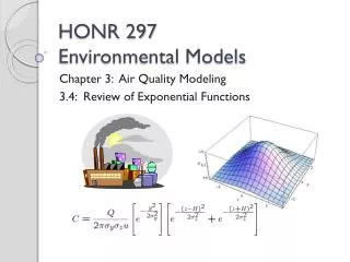
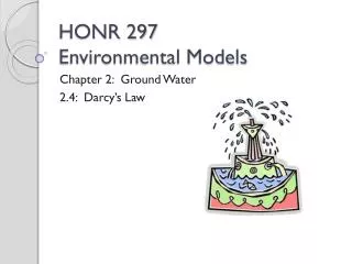
HONR 297 Environmental Models. Chapter 2: Ground Water 2.7: Water Table Contour Maps. Images Courtesy: Charles Hadlock , Mathematical Modeling in the Environment. Hydraulic Head Revisited.

E N D
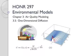
HONR 297Environmental Models Chapter 2: Ground Water 2.7: Water Table Contour Maps Images Courtesy: Charles Hadlock, Mathematical Modeling in the Environment
Hydraulic Head Revisited • From our work with Darcy’s Law and the interstitial velocity equation, it should be clear that a key to ground water investigation is the hydraulic head. • The general method to determine groundwater head levels is to drill several test wells and measure depths to ground water to determine the water table elevation via known horizontal datum levels! Courtesy USGS: http://ga.water.usgs.gov/edu/earthgwwells.html
Water Table Contour Map • Once the data from the test wells is collected, the corresponding head information is usually put into a water table contour map, such as the one shown in Figure 2.20 of our text (p. 39). Courtesy: Charles Hadlock, Mathematical Modeling in the Environment
Water Table Contour Map • In a fashion similar to topographic maps, which display points of equal elevation via contour lines, water table contour maps show points of equal head value via contour lines! Courtesy: Charles Hadlock, Mathematical Modeling in the Environment
Water Table Contour Map • Remark: Usually, water table contour maps are constructed from test well head levels by means of interpolation and extrapolation. • The general topography of the land surface above the water table may also be taken into account (especially for a shallow ground water aquifer). Courtesy: Charles Hadlock, Mathematical Modeling in the Environment
Key Fact! • When working with water table contour maps, it is a good idea to keep the following fact in mind: • Water Table Contour Map Key Fact: At any point, the ground water always* tends to flow in a direction that is perpendicular to the head contour at that point. • Reason: Think of a marble rolling down the side of a hill – it will always want to move down the hill in the direction that is always as steep or directly downward as possible. • Mathematically we say the marble is following the path of steepest descent, which turns out to be perpendicular to topographic contour lines. • Ground water behaves in the same way – it responds to gravity and wants to follow the steepest or quickest path down the water table. • In the rest of Chapter 2 we will assume that the Key Fact holds – i.e. the flow of groundwater will be perpendicular to contour lines. • *The path of the groundwater may be blocked or deflected in some portion of the aquifer – similar to a marble rolling downhill and hitting a tree. We will assume in what follows that this does not happen. Courtesy: Charles Hadlock, Mathematical Modeling in the Environment
Example 1 • Consider the hydraulic head contour map shown in Fig. 2.2 of our text (p. 41). Assume the aquifer under consideration has a hydraulic conductivity of 50 ft/day and a porosity of 25%. Assuming that a source of contamination exists at the point marked X, determine • Which of the three wells W1, W2, or W3 will most likely be directly affected. • How long will it take for the contaminated ground water to travel from the point X to the affected well? Courtesy: Charles Hadlock, Mathematical Modeling in the Environment
Example 1 • Solution: • (a) Since the head levels decrease as we move to the right, using the key fact, we can sketch a flow line starting at X and ending at W3 (see Fig. 2.23 in text). Courtesy: Charles Hadlock, Mathematical Modeling in the Environment
Example 1 Courtesy: Charles Hadlock, Mathematical Modeling in the Environment
Example 1 Courtesy: Charles Hadlock, Mathematical Modeling in the Environment
Example 1 • Solution: • (b) Using the ground water flow line we drew in part (a), along with the water table contour lines, we can estimate travel time via the interstitial velocity equation and the relationship • time = distance/velocity. • First, break the flow path into segments which are determined by the contour lines, starting point X, and ending point W3. • In this case, we will have five segments! • Our goal is to compute travel time of the groundwater for each of the five segments. Courtesy: Charles Hadlock, Mathematical Modeling in the Environment
Example 1 S1 S2 S3 S4 Courtesy: Charles Hadlock, Mathematical Modeling in the Environment S5
Example 1 • Recall that ν = (K i)/η. • We are given • K = 50 ft/day • η = 0.25. • From the water table contour map we can find i = Δh/L for each of the segments 2, 3, and 4. • Δh is found from the given contour levels and L can be measured off of the map using the given scale!
Example 1 • For segments 1 and 5, we cannot measure Δh from the given information, so we will assume the hydraulic gradient i doesn’t change drastically from one point to nearby points. • Therefore, assume that the hydraulic gradients in segments 1 and 5 are the same as the hydraulic gradient in adjacent segments.
Example 1 • Let d = length of a given segment. • Then in each calculation that follows, L = d. • Also, let t = travel time in a given segment. • Segment 2: • d = 460 ft • i = Δh/L = (85 ft - 80 ft)/460 ft = 5/460 ≈ 0.011 • ν = (K i)/η = ((50 ft/day)(5/460))/0.25 ≈ 2.2 ft/day • t = d/ ν = (460 ft)/(((50 ft/day)(5/460))/0.25) ≈ 209 days.
Example 1 • Segment 1: • d = 170 ft • i = 5/460 ≈ 0.011 (from segment 2) • ν = (K i)/η = ((50 ft/day)(5/460))/0.25 ≈ 2.2 ft/day • t = d/ ν = (170 ft)/(((50 ft/day)(5/460))/0.25) ≈ 77 days. • Find the time ground water takes to flow along segments 3, 4, and 5 … • Our findings can be summarized in a table:
Using Excel for Ground Water Travel Time • We can set up a table in Excel to automate the process used for the calculations of travel time in each segment. • Hadlock suggests a set-up on page 43.
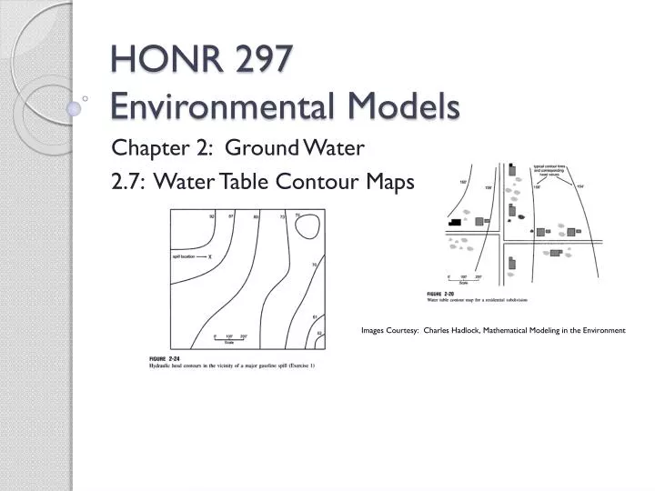
Example 2 • Consider the situation described by Fig. 2.24. The contour lines represent estimated contours of hydraulic head in a shallow aquifer composed chiefly of coarse sand. If a major gasoline spill onto the ground occurs at point X, as shown in Fig. 2.24, and some of the gasoline seeps down to the water table, indicate on the diagram its likely migration path with the ground water, and estimate how long it might take for the first traces of dissolved gasoline to reach the boundary of the region shown in the figure. Pick representative values of hydrologic parameters you need from Table 2.1. If you need to make any additional assumptions, be sure to explain what you do. Courtesy: Charles Hadlock, Mathematical Modeling in the Environment
Example 2 Courtesy: Charles Hadlock, Mathematical Modeling in the Environment
Resources • Charles Hadlock, Mathematical Modeling in the Environment, Section 2.7 • Figures 2.20, 2.21, 2.22, 2.23, and 2.24 used with permission from the publisher (MAA). • USGS: • http://ga.water.usgs.gov/edu/earthgwwells.html