Download
1 / 34
340 likes | 345 Views
Impedance measurements with the ILC prototype cavity. Dr G. Burt Cockcroft Institute Lancaster University. P. Goudket, P. McIntosh, A. Dexter, C. Beard, P. Ambattu. Modal Calculations in MAFIA. Lower Order Modes, 2.8 GHz. High impedance monopole modes are not a problem.

E N D
Impedance measurements with the ILC prototype cavity Dr G. Burt Cockcroft Institute Lancaster University P. Goudket, P. McIntosh, A. Dexter, C. Beard, P. Ambattu
Modal Calculations in MAFIA Lower Order Modes, 2.8 GHz High impedance monopole modes are not a problem Operating and Same Order modes at 3.9 GHz Narrowband dipole modes seen up to 18 GHz High dipole impedances seen at 10 GHz and 13 GHz 1st Dipole passband Trapped 5th dipole passband at 8 GHz
Crab Cavity Prototype • Model fabricated at DL and used to evaluate: • Mode frequencies • Cavity coupling • HOM, LOM and SOM Qe and R/Q • Modular design allows evaluation of: • Up to 13 cells. • Including all mode couplers.
The cells are not squashed and are cylindrically symmetric. Two small discs is inserted into each cell in order to polarise the cavity. Prototype Cell Shape
Slater’s theorem Slater’s paper [[i]] states, in a cavity, the fractional change in frequency is proportional to the fractional change in stored energy. This can be used to characterise a standing wave cavity by introducing a small perturbation to the cavity and observing the change in frequency as the perturbation is induced. The change in cavity energy by a perturbation to the electric field can be calculated to be equal to [i] L.C. Maier, J.C. Slater, Field Strength Measurements in Resonant Cavities, Journal of Applied Physics, 23 (1), 1952 Perturbation Theory
A perturbing object placed within a cavity will change the resonant frequency of that structure proportionally to the field on the surface of the perturbing object. Bead Coupler offset VNA Frequency without bead: 3.98539GHz Frequency with perturbing bead: 3.98554GHz -> 150kHz frequency shift 2mm radius bead Non-Resonant Perturbation Technique By pulling a bead through the cavity we can map the fields within the cavity as the frequency perturbation is proportional to the fields at that position.
Non-spherical beads can distinguish between longitudinal and transverse field components. Different type of beads • Dielectric beads allow the perturbation to only affect the electric field and not the magnetic field. • Metal beads are perturbed by both fields.
Frequency shift vs. Phase shift It is often a slow process to use frequency shifts to characterise a cavity so instead it is possible to work out the frequency shift from the phase shift at a fixed frequency. However with large perturbations the frequency calculated from the phase shift can often be smaller than the actual frequency shift as the relation moves out of the linear region.
LOM measurements Monopole modes can be measured by directly measuring the frequency shift (or phase) by pulling a metallic circular bead along the cavity axis as the Ez field strongly dominates in this region. As can be seen we achieved good agreement with simulations for R/Q.
Dipole Bead-pull results • If we pull a dielectric bead along the axis we can find the transverse E field on axis • We can then use this to separate the transverse E and B fields perturbing a metal bead. • Hence we can calculate the R/Q from Panofsky Wenzel theorem.
Alternatively we can use a metal needle to perturb the cavity. Needle measurements • According to Pierce a needle will strongly perturb electric fields aligned with it and weakly perturb perpendicular electric fields and magnetic fields. • The other fields will however cause small errors.
For the HOM’s, things become more complicated. The bead-pull doesn’t give you the sign of the field so that has to be known. The reflections at the end of the beam-pipe cause trapped modes. Higher Order Modes
Wire Measurements Technique • Technique employed extensively on X-band structures at SLAC. • Bench measurement provides characterisation of: • mode frequencies • kick factors • loss factors A pulse travelling along a wire has a similar field profile to a relativistic bunch. The wire can move off axis to induce dipole modes.
Transmission Theory A wire through a uniform reference tube can be regarded as a transmission line characterised by Ro , Lo and Co A wire through the cavity under investigation is modelled with an additional series impedance Zll / l The impedance Zll is large close to each cavity mode . One measures reflections of a wave passing along the wire for the cavity (DUT) with respect to the plain tube (Ref) then determines Zlland hence kloss from theequations opposite. As q is measured as a function of frequency one obtains a loss factor at each frequency where Zll is large i.e. for each mode.
Impedance Matching A conical broadband impedance transformer and a series of quarter wave resonators were used to provide a good match between the DUT and the RF source. There is some disagreement in the community whether good matching is required or not so we erred on the side of caution
Perturbation by the wire The presence of the wire however perturbs the fields of the cavity and will shift the frequency and R/Q. This makes this technique only applicable to dipole, quadropole and higher azimuthal order modes. At larger wire offsets errors creep into the dipole measurements
Wire Measurements Technique We use an on-axis measurement as our reference and off-axis measurements as the DUT. By observing how the coupling impedance varies with offset we can ascertain the mode order. This technique is a fast method of measuring the impedance over a large bandwidth.
Operating Mode Measurements The coupling impedance was measured for 3 and 9 cell cavities and was in good agreement with bead-pulls and MAFIA simulations. We investigated how the measurements varied with wire offset. As we can see the R/Q decreases at large offsets due to the wire perturbation. In addition there are large error bars at low offsets due to the percentage uncertainty in the wire position.
The monopole modes resonant frequency was found to alter sizably as the wire was moved off-axis causing to cause errors in nearby dipole modes as the reference and DUT transmission will differ. Monopole modes
The measurements were repeated several times over several days in order to ascertain repeatability of the measurements. Repeatability It is believed that due to the construction of the cavity that as the cavity was moved about cell misalignments moved causing the impedance to change. If the cavities were kept still the measurements were fairly repeatable.
Full System Prototype At present we have built and are measuring the prototypes of the UK SOM coupler and power coupler and the SLAC HOM and LOM couplers to verify the full system.
Coupler Measurements The external Q of the couplers were measured using the transmission from a calibrated probe of known Qe. This is more accurate for high Qe’s than a reflection measurement.
Power Coupler Prototype Measurements In the spring 2007 I made measurements of power coupler and SOM coupler prototypes in order to verify the codes. 3 cell cavities were used to preserve field flatness. There was some issues with metallisation of the window which have now been rectified.
Dipole modes damping by SOM coupler The SOM coupler used was not the coupler modelled by SLAC. The CI SOM coupler was manufactured instead. This is not the full external Q, just the contribution from the SOM. After adjustment the operating mode Qe is 8.84E9
LOM Coupler Prototype external Q measurements The LOM coupler was found to give good agreement with both MWS and Omega 3P simulations. However it doesn’t meet the damping requirements for the ILC.
HOM coupler The HOM coupler is the most complex of all 4 couplers and a large amount of time was spent analysing it. Modes up to 7.8 GHz were found. Modes not found assumed to flow out of the beam-pipes.
HOM Coupler The filter was made adjustable to investigate manufacturing errors. The gap sensitivity was found to be 0.135 MHz/ micron. The measurements were found to give good agreement with the SLAC simulations (courtesy of Z. Li and L. Xiao)
A few LHC crab cavity simulations G. Burt, R. Calaga
Short Range Wakes ECHO 2D was used to calculate the longitudinal short range wakes in Rama’s design for the LHC cavity. The transverse wake was calculated analytically.
Dipole HOMs Then MAFIA’s 2D eigensolver was used to look at the dipole modes up to 3 GHz. Some of these modes will be highly perturbed by the boundary conditions at the end of the beampipes.
Beam-pipe LOM coupler The damping of the two LOM’s were investigated using a KEK-B style beam-pipe LOM coupler. The inner diameter was 10cm and the penetration was varied. This currently doesn’t have a notch filter and is just a basic investigation. If we go for this design it means that we need a large beam-pipe to fit the coupler which will reduce the maximum voltage.
LOM coupler modelling 4mm A LOM coupler can be coaxial hook type LOM coupler can get very low external Q’s. Waveguide LOM couplers are also effective. 27mm 12mm ILC Crab cavity Single cell Qe LOM=150 72mm 7mm 25mm
SOM Waveguide Coupler A waveguide SOM coupler was investigated and achieved a Qe of 4.5x10³. The WG was positioned 40 mm from the cavity. A scheme of a WG power coupler, two WG SOM/HOM couplers cut-off to the fundamental and a beam-pipe, coaxial or WG LOM coupler on the other side could be a potential damping scheme. The power coupler would have to also extract the other mode in the 1st dipole pass-band.