Download
1 / 61
1.06k likes | 2.27k Views
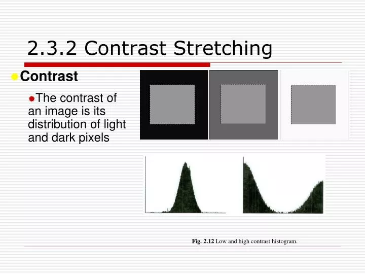
2.3.2 Contrast Stretching. Contrast The contrast of an image is its distribution of light and dark pixels. Fig. 2.12 Low and high contrast histogram. Contrast Stretching. Contrast stretching Clipping thresholding. Contrast Stretching. Contrast Stretching, a = 80, b= 160. Original Image.

E N D
2.3.2 Contrast Stretching • Contrast • The contrast of an image is its distribution of light and dark pixels Fig. 2.12 Low and high contrast histogram.
Contrast Stretching • Contrast stretching • Clipping • thresholding
Contrast Stretching Contrast Stretching, a = 80, b= 160
Original Image Basic Contrast Stretching Original Image End-in Search Contrast Stretching
Contrast Stretching Original Image Convert Image
Red Green Blue
/******************************************** • * Func: auto_contrast_stretch • * Desc: performs basic contrast stretching on an image • * Params: source - pointer to source image • * cols - number of columns in the image * rows - height of image * • ********************************************* • void auto_contrast_stretch(image_ptr source, int cols, int rows) • { • long i; /* loop variable */ • long number_of_pixels; /* total number of pixels in image */
long histogram[256]; /* image histogram */ • unsigned char LUT[256]; /* Look-up table for point process */ • int lowthresh, highthresh; /* lower and upper thresholds */ • float scale_factor; /* scaling factor for contrast stretch */ • /* compute histogram */ • number_of_pixels = (long)cols * rows; • for(i=0; i<256; i++) • histogram[i]=0; • for(i=0; i<number_of_pixels; i++) • histogram[source[i]]++;
/* compute low and high thresholds */ • for(i=0; i<256; i++) • if(histogram[i]) { • lowthresh = i; • break; • } • for(i=255; i>0; i--) • if(histogram[i]) { • highthresh = i; • break; • }
printf("Low threshold is %d High threshold is %d\n", • lowthresh,highthresh); • /* compute new LUT */ • for(i=0; i<lowthresh; i++) • LUT[i]=0; • for(i=255; i>highthresh; i--) • LUT[i]=255;
scale_factor = 255.0 / (highthresh-lowthresh); • for(i=lowthresh; i<=highthresh; i++) • LUT[i]=(unsigned char)((i - lowthresh) * scale_factor); • /* transfer new image */ • for(i=0; i<number_of_pixels; i++) • source[i] = LUT[source[i]]; • }
2.3.3 Intensity transformations • Digital negative • Applications • Display of medical images • Produce negative prints of images • Intensity level slicing • Applications : • Segmentation of certain gray level regions
Intensity transformations • Intensity transformation • Convert an old pixel into a new pixel based on some predefined function • Implemented with simple look-up tables • Simple transformation • Null transform • new pixel = old pixel • Image negative • y = -x+255 • Gamma correction function • Brightness of an image can be adjusted with a gamma correction transformation
Intensity transformations • Posterizing • reduces the number of gray levels in an images • Thresholding results when number of gray levels is reduced to 2. • A bounced threshold reduces the thresholding to a limited range and treats the other input pixels as null transformation • Figure 2.18(pp.63) Fig. 2.18 (a) 8-Level posterize transformation; (b) posterized image; (c) threshold transformation; (d) threshold image; (e) bounded threshold; (f) bounded threshold image.
Original gamma=0.45 gamma=2.20 Intensity transformations • Gamma correction
Intensity Transformation • Intensity Transformation • Intensity transformation is a point process that converts an old pixel into a new pixel base on some predefined function. This transformation is implemented with the LUT with ease. • Gamma Correction
Intensity transformations Fig. 2.16 (a) Gamma collection transformation with gamma=0.45; (b) gamma collected image; (c) gamma collection transformation with gamma=2.2; (d) gamma collected image. Fig. 2.15 (a) Null transformation; (b) image; (c) negative transformation; (d) negative image. Page 60. 참조
Intensity transformations Fig. 2.17 (a) Contrast stretch transformation; (b) contrast stretched image; (c) Contrast compression transformation; (d) contrast compressed image. Fig. 2.18 (a) 8-Level posterize transformation; (b) posterized image; (c) threshold transformation; (d) threshold image; (e) bounded threshold; (f) bounded threshold image. Page 62. 참조
Intensity transformations Fig. 2.19 (a) 2-bit bit-clipping transformation; (b) resulting image. Fig. 2.21 (a) Iso-intensity contouring transformation; (b) contoured image. Fig. 2.20 Bit clipped image contrast stretched. Page 64. 참조
Intensity tranformations Fig. 2.22 (a) Range-highlighting transformation; (b) resulting image. Fig. 2.23 (a) Solarize transformation using a threshold of 150; (b) solarize image. Page 65. 참조
Fig. 2.24 (a) First parabola transformation; (b) transformed image; (c) second parabola transformation; (d) second transformed image.
HW – 03 a) Plot กราฟ histogram
สจพ 2.4 Frequency-based Operations Fourier Transform DI&SP MTCT
Spatial Frequency • Efficient data representation • Provides a means for modeling and removing noise • Physical processes are often best described in “frequency domain” • Provides a powerful means of image analysis
What is spatial frequency? • Instead of describing a function (i.e., a shape) by a series of positions • It is described by a series of cosines • Fourier series • Fourier Transform
สจพ 1-D Fourier Transform DI&SP MTCT
Our starting place is the observation that a periodic function may be written as the sum of sines and cosines of varying amplitudes and frequencies.
it is possible to form any function as a summation of a series of sine and cosine terms of increasing frequency • For example, in figure we plot a function, and its decomposition into sine functions.
We take the first three terms only (blue, green, red) to provide the approximation of the original function (purple). • The more terms of the series we take, the closer the sum will approach the original function.
Original function (purple) sines and cosines (1) where (2) Fourier coefficient Equations 1 and 2 are called Fourier transform pairs, and they exist if f(t) is continuous and integrable, and F(k) is integrable. These conditions are usually satisfied in practice.
f(t) => time-domain I 1 2 3 4 1 F(u) => frequency-domain 3 II 4 2
Any function can be represented in 2formats: • 1) time-domain representation, f(t), or spatial domain, f(x), and • 2) frequency-domain representationor Fourier domain, F(u) • In other words, any space ortime varying data can be transformed into a different domain called the frequencyspace.
Time-domain Frequency-domain
FT properties: If F(u) and G(u)are FT of function f(t) and g(t), respectively, • Time scaling • Frequency scaling
Time shifting • Frequency shifting
Convolution theorem • Correlation theorem
สจพ 2-D Fourier Transform DI&SP MTCT
แนวความคิดของการแปลงฟูเรียร์สามารถนำมาใช้กับฟังก์ชั่นหรือสัญญาณ 2 มิติ เช่น ภาพ ซึ่งจะเป็นการแปลงฟังก์ชั่นบน spatial domain (รูปภาพ) ไปเป็น frequency domain สมการคณิตศาสตร์แสดงความสัมพันธ์นี้เป็นดังนี้ IFT FT
ภาพแสดงความสัมพันธ์ระหว่างภาพใน spatial domain และความถี่ใน frequency (or Fourier) domain
พบว่าระยะถี่-ห่างทางตำแหน่งในภาพ (x-y ใน spatial domain) จะแปลงไปเป็นจุดใน frequency domain(u-v) • โดยบริเวณที่มีระยะห่าง (ซึ่งมีความถี่ทางตำแหน่งต่ำ) เช่น บริเวณตัวบ้านรวมทั้งหน้าต่าง-ประตู จะไปอยู่ในตำแหน่งที่ใกล้จุดกำเนิด • และในทางกลับกันบริเวณที่มีระยะถี่ (ซึ่งมีความถี่ทางตำแหน่งสูง) เช่น บริเวณที่มีลวดลายบนหลังคาบ้าน จะไปอยู่ในตำแหน่งที่ไกลจุดกำเนิดออกไป