Download

1 / 24
240 likes | 444 Views
Multi-sample structural equation models with mean structures. Hans Baumgartner Penn State University. Measurement invariance. measurement invariance:

E N D
Multi-sample structural equation models with mean structures Hans Baumgartner Penn State University
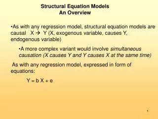
Measurement invariance • measurement invariance: “whether or not, under different conditions of observing and studying phenomena, measurement operations yield measures of the same attribute” (Horn and McArdle 1992); • frequent lack of concern for, or inappropriate examination of, measurement invariance in cross-national research; • this is problematic because in the absence of measurement invariance cross-national comparisons may be meaningless;
Measurement model Let xg be a p x 1 vector of observed variables in country g, xg an m x 1 vector of latent variables, dg a p x 1 vector of unique factors (errors of measurement), tg a p x 1 vector of item intercepts, and Lg a p x m matrix of factor loadings. Then xg = tg + Lgxg + dg The means part of the model is given by mg = tg + Lgkg and the covariance part is given by Sg = LgFgLg ' + Qg
d d d d d d d d q44 q88 q66 q77 q33 q22 q11 q55 j21 j11 j22 1 x1 x2 k1 k2 1 l2 l3 l4 1 l6 l7 l8 0 t2 t3 t4 0 t6 t7 t8 x1 x2 x3 x4 x5 x6 x7 x8 d1 d2 d3 d4 d5 d6 d7 d8
Model identification • covariance part: the latent constructs have to be assigned a scale in which they are measured; this is done by choosing a marker item for each factor and setting its loading to one; • means part: two possibilities • the intercepts of the marker items are fixed to zero (which equates the means of the latent constructs to the means of their marker variables, mmg = kg); • the vector of latent means is set to zero in the reference country and one intercept per factor is constrained to be equal across countries; • although these constraints help with identifying the model, in general they are not sufficient for meaningful cross-national comparisons;
Types of invariance • configural invariance: the pattern of salient and nonsalient loadings is the same across different countries; • metric invariance: the scale metrics are the same across countries; L1 = L2 = ... = LG • scalar invariance: in addition to the scale metrics the item intercepts are the same across countries; t1 = t2 = ... = tG
Configural invariance 1 1 x1 x1 x2 x2 x6 x6 x1 x1 x2 x2 x3 x3 x5 x5 x7 x7 x4 x4 x8 x8
Metric invariance 1 x1 x2 x6 x1 x2 x3 x5 x7 x4 x8 1 x1 x2 x6 x1 x2 x3 x5 x7 x4 x8
Scalar invariance 1 x1 x2 x6 x1 x2 x3 x5 x7 x4 x8 1 x1 x2 x6 x1 x2 x3 x5 x7 x4 x8
Types of invariance (cont’d) • factor (co)variance invariance: factor covariances and factor variances are the same across countries; F1 = F2 = ... = FG • error variance invariance: error variances are the same across countries; Q1 = Q2 = ... = QG
Linking the types of invariance required to the research objective
Full vs. partial invariance • measurement invariance of a given type (e.g., metric, scalar) may not be fully satisfied; • partial measurement invariance as a “compromise” between full measurement invariance and complete lack of invariance (Byrne et al. 1989); • issue of the minimal degree of partial measure-ment invariance necessary for cross-national comparisons to be meaningful (Steenkamp and Baumgartner 1998);
Partial measurement invariance • for identification purposes, one item per factor has to have invariant loadings and intercepts (marker item); the marker item has to be chosen carefully; • at least one other invariance constraint on the loadings/ intercepts is necessary to ascertain whether the marker item satisfies metric/scalar invariance; • Cheung and Rensvold (1999) proposed the factor-ratio test in which all possible pairs of items are tested for metric invariance and sets of invariant items are identified; • an alternative is to start with the fully invariant model of a given type and relax invariance constraints based on significant modification indices, changes in alternative fit indices, and expected parameter changes;
Assessing metric invariance across different groups • choose a marker item for each factor • (e.g., based on reliability or other considerations; if it later turns out that the marker item does not satisfy metric or scalar invariance, a different marker item may have to be chosen) • compare the configural with the full metric invariance model; • use Bonferroni-adjusted modification indices, changes in alternative fit indices, and expected parameter changes to free loadings that are not invariant; the final model should fit as well as the configural model; • cross-validate the model, if possible;
Assessing scalar invariance across different groups • compare the final (partial) metric invariance model with the full (or initial) scalar invariance model; • use Bonferroni-adjusted modification indices, changes in fit indices, and expected parameter changes to free item intercepts that are not invariant; the final model should fit as well as the final (partial) metric invariance model; • cross-validate the model, if possible;
Illustration • 393 Austrian and 1181 U.S. respondents completed the Satisfaction with Life Scale (SWLS; Diener et al. 1985), which is a well-known instrument used to assess the cognitive component of subjective well-being. The scale consists of the following five items: • In most ways my life is close to my ideal. • The conditions of my life are excellent. • I am satisfied with my life. • So far I have gotten the important things I want in life. • If I could live my life over, I would change almost nothing. • Respondents indicated their agreement or disagreement with these statements using the following five-point scale: 1 = strongly disagree, 2 = disagree, 3 = neither agree nor disagree, 4 = agree, and 5 = strongly agree. • Perform an analysis of measurement invariance on the SWLS and test whether Austrian or American respondents are more satisfied with their lives (if possible).
d d d d d d d d q44 q88 q66 q77 q33 q22 q11 q55 j21 j11 j22 1 x1 x2 k1 k2 1 l2 l3 l4 1 l6 l7 l8 0 t2 t3 t4 0 t6 t7 t8 x1 x2 x3 x4 x5 x6 x7 x8 d1 d2 d3 d4 d5 d6 d7 d8
GROUP: AUSTRIA Observed Variables: ls1 ls2 ls3 ls4 ls5 Raw data from file ls-aut.dat Sample Size: 393 Latent Variables: LS Relationships: ls1 = CONST + LS ls2 = CONST + LS ls3 = 1*LS ls4 = CONST + LS ls5 = CONST + LS LS = CONST GROUP: USA Observed Variables: ls1 ls2 ls3 ls4 ls5 Raw data from file ls-usa.dat Sample Size: 1181 Latent Variables: LS Relationships: LS = CONST Set the path LS -> ls5 free Set the path CONST -> ls5 free Set the Error Variance of ls1 free Set the Error Variance of ls2 free Set the Error Variance of ls3 free Set the Error Variance of ls4 free Set the Error Variance of ls5 free Set the Variance of LS free Options mi End of Problem
Bagozzi, Baumgartner, and Pieters (1998) 0.31 (7.4) dieting volitions dieting behaviors .14 (3.6) .20 (7.4) .36 (6.8)d -.07 (-.6) .54 (4.9)b positive goal-outcome emotions positive anticipated emotions .61 (7.7)a,b .29 (3.1)c,d .16 (4.4) goal achievement .16 (4.0) negative anticipated emotions negative goal-outcome emotions -.18 (-2.3)a,c -.46 (-8.7)b,d .08 (.9) .56 (3.7)a .24 (8.7) exercising volitions exercising behaviors .07 (1.9) 0.11 (3.4) .33 (5.3)b a men wanting to lose weight b women wanting to lose weight c men wanting to maintain their weight d women wanting to maintain their weight c2(110)=150.51 RMSEA=.030 CFI=.94 TLI=.92