Minimum Cost Flows

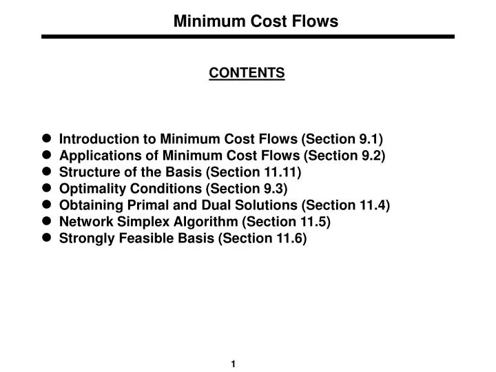
1. Minimum Cost Flows CONTENTS • Introduction to Minimum Cost Flows (Section 9.1) • Applications of Minimum Cost Flows (Section 9.2) • Structure of the Basis (Section 11.11) • Optimality Conditions (Section 9.3) • Obtaining Primal and Dual Solutions (Section 11.4) • Network Simplex Algorithm (Section 11.5) • Strongly Feasible Basis (Section 11.6)

2. Minimum Cost Flow Problem Determine a least cost shipment of a commodity through a network in order to satisfy demands at certain nodes from available supplies at other nodes. Arcs have capacities and cost associated with them. -15 2 2 4 2 3 1 5 4 4 5 7 1 10 10 6 3 6 6 3 5 -5 • Distribution of products • Flow of items in a production line • Routing of cars through street networks • Routing of telephone calls

3. Minimum Cost Flow Problem (contd.) Mathematical Formulation: where • Supply nodes (b(i) > 0); Demand nodes (b(i) < 0),Transhipment nodes (b(i) = 0) • Mass balance constraints (flow out - flow in = supply/demand) • Flow bound constraints (lower and upper bound constraints)

4. Assumptions • All data (cost, supply/demand, capacity) are integral. • The network is directed. • The sum of supplies equals the sum of demands, and the problem admits a feasible flow. • The network contains an uncapacitated directed path between every pair of nodes. • All arc costs are non-negative.

5. p1/m1 r1/m1 p1/m2 r1/m2 r1 p2/m1 r1/m3 p2/m2 r2/m1 r2 p2/m3 r2/m2 p 1 Plant nodes Plant/model nodes Retailer/model nodes Retailer nodes p 2 Distribution Problems A car manufacturer has several manufacturing plants and produces several car models at each plant that is shipped to various retailers. The manufacturer must determine the production plan for each model and shipping pattern that minimizes the overall cost of production and transportation.

6. ……….…. n 2 1 3 n-1 Airplane Hopping Problem • A hopping flight visits the cities 1, 2, 3, … , n, in a fixed sequence. • The plane can pickup passengers at any node and drop them off at any other node. • Let bij denote the number of passengers available at node i who want to go to node j and let fij denote the fare for such passengers. • Determine the pickup policy to maximize the total fare.

7. b(i) b(j) cij uij or i j b24 b14 b34 1-4 2-4 3-4 -f24 -f34 b13 1-3 -f14 cost -f13 b12 b23 2-3 1-2 -f12 -f23 1 2 3 4 p p p capacity Airplane Hopping Problem (contd.)

8. Linear Programs with Consecutive Ones Consider the following linear programming problem: Minimize cx subject to x  0 Subtract surplus variables y to convert inequalities to equations.

9. Linear Programs with Consecutive Ones (contd.) Minimize cx subject to x, y  0 Subtract ith constraint from the (i+1)th constraint.

10. Linear Programs with Consecutive Ones (contd.) Minimize cx subject to x, y  0 This is the formulation of a minimum cost flow problem.

11. Examples of LP’s with Consecutive Ones • Nurse scheduling • Telephone operator scheduling • Equipment replacement • Employment scheduling • Optimal capacity planning

12. (15,40) 4 2 (25,30) (15,30) (45,10) 1 (35,50) (45,60) (35,50) 3 5 (25,20) Properties of the Constraint Matrix • Any variable xij has a +1 in the ith row and a -1 in the jth row. • The rows of the constraint matrix are linearly dependent. • The rank of the constraint matrix is at most (n-1).

13. Properties of the Basis (contd.) THEOREM: There is a one-to-one correspondence between basis of the minimum cost flow problem in G and spanning trees of G. Triangularity property (or spanning tree property) allows us to speedup simplex computations substantially. Computing Basic Feasible Solutions: BxB = b Determining Simplex Multipliers: pB = cB

14. Spanning Tree Structure The minimum cost flow problem is a special case of the bounded variable linear programming problem. Basic Arcs (T): Arcs in the spanning tree. Nonbasic Arcs at Lower Bounds (L): Arcs not in the spanning tree with zero flow. Nonbasic Arcs at Upper Bounds (U): Arcs not in the spanning tree at their upper bounds. (T, L, U): Basis structure or Spanning tree structure. Feasible spanning tree structure Optimal spanning tree structure

15. Optimality Conditions THEOREM: A spanning tree structure (T, L, U) is an optimal spanning tree structure of the minimum cost flow problem if it is feasible and there exists a vector of dual variables (called, node potentials) p such that the arc reduced costs satisfy the following conditions: = 0 for all (i, j)  T,  0 for all (i, j)  L,  0 for all (i, j)  U. where = cij - p(i) + p(j). PROOF: These are the LP optimality conditions specialized for the minimum cost flow problem.

16. Maintaining a Spanning Tree Structure • We consider the spanning tree hanging from a specially designated node, called the root. • We associate three indices with each node i of the tree: • pred(i): The predecessor index. Maintains the parent of node i in the tree. • depth(i): The depth index. Maintains the number of arcs from node i to the root node. • thread(i): The thread index. Defines a depth-first traversal of the tree.

17. 1 2 3 5 6 7 4 8 9 Maintaining a Spanning Tree Structure (contd.)

18. i p(i) i p(i) p(j) = p(i) + cji j p(j) = p(i) - cij j Computing Node Potentials The node potentials p are computed using the fact that = 0 for every basic arc (i, j)  T where = cij - p(i) + p(j).

19. Computing Node Potentials (contd.) 1 0 1 5 p(i) -5 2 2 1 3 2 1 -2 -3 3 5 3 5 cij 1 4 1 3 6 -7 7 -2 6 -1 4 3 7 4 p(j)

20. Computing Node Potentials (contd.) procedure computing node-potentials; begin p(1) : = 0; j : = thread(1); while j  1 do begin i : = pred(j); if (i, j)  A thenp(j) : = p(i) - cij; if (j, i)  A thenp(j) : = p(i) + cji; j : = thread(j); end; end;

21. i b(i) b(i) i xij = -b(j) xij = b(j) b(j) j j b(j) Computing Arc Flows Suppose that there is a leaf node j with supply/demand b(j).

22. 1 i 5 10 3 2 xij 5 5 15 10 j 4 7 5 6 Computing Arc Flows (contd.) 15 1 b(i) i 0 -20 3 2 j 4 7 5 6 b(j) 5 5 -15 10

23. Computing Arc Flows (contd.) Procedure when U = Ø : procedure computing arc-flows; begin b(i) : = b(i) for all i  N; for each (i, j)  L do set xij : =0; T : = T; while T {1} do begin select a leaf node j in T; i : = pred(j); if (i, j)  T then xij : = -b(j); else xji : = b(j); add b(j) to b(i); delete node j and the arc incident to it from T; end; end;

24. Computing Arc Flows (contd.) Procedure when U Ø: for each arc (i, j)  U do set xij := uij, subtract uij from b(i) and add uij to b(j); procedure computing arc-flows;

25. Network Simplex Algorithm algorithm network-simplex; begin determine the initial feasible tree structure (T, L, U); let x be the flow and p be the node potentials; while some nontree arc violates its optimality condition do begin select an entering arc (k, l) violating its opt. condition; add arc (k, l) to the tree and determine the leaving arc; perform a tree update, and update x and p; end; end;

26. 2 b(2) < 0 6 b(6) < 0 3 b(3) < 0 1 7 b(7)  0 b(4)  0 4 5 b(5)  0 Obtaining initial Basis Structure

27. Entering Arc Selection Optimality Conditions:  0 for every arc (i, j)  L;  0 for every arc (i, j)  U; Eligible Arcs: < 0 for any arc (i, j)  L; > 0 for any arc (i, j)  U; Violation of an eligible arc:

28. Pivot Rules • Dantzig’s Pivot Rule: Select the arc with the maximum violation as the entering arc. • First Eligible Arc Pivot Rule: Select the first eligible arc found as the entering arc. • Candidate List Pivot Rule: • Major iteration: Construct the candidate list. • Minor iteration: Select an entering arc from the candidate list.

29. Pivot Operation 1 • Determine the pivot cycle W defined by the entering arc. • Determine the maximum flow d that can be augmented along W. • Example: d = min{u43-x43, u32-x32, u25-x25, x56, u69-x69, u94-x94} • Degenerate iteration (d =0) • Nondegenerate iteration (d >0) • Update the flow. • Determine the leaving arc. Apex 2 3 5 6 7 4 Entering arc 8 9

30. Pivot Operation 1 • Get the new spanning tree. • Update the node potentials. • Update the tree indices. 2 3 5 6 7 4 Entering arc 8 9

31. p(j) p(i) xij b(i) b(j) (cij,uij) i j -8 -3 (5,7) 5 j 4 4 2 2 i (3,5) (3,8) 6 (2,2) 1 -9 -9 6 6 (5,4) 9 0 (2,3) 1 1 3 (2,3) 4 (4,6) 5 5 3 3 3 (4,3) -5 -2 Example of Network Simplex Algorithm

32. 4 4 2 2 6 6 1 1 3 3 Example of Network Simplex Algorithm (contd.) -8 -8 -3 -3 4 5 4 5 6 7 -11 -10 0 0 3 2 5 4 5 5 2 -7 -2 -6 -2

33. Running Time Analysis • Time per Iteration: • Update the flow (takes O(n) time). • Update the node potentials (takes O(n) time). • Update the tree indices (takes O(n) time). • Number of Iterations: • Number of non-degenerate pivots: O(mCU) • Number of degenerate pivots: No bound is possible