Download
1 / 24
240 likes | 342 Views
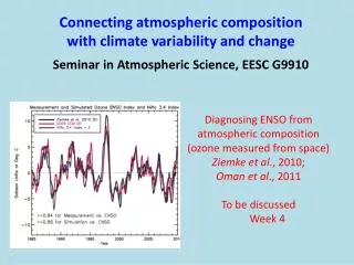
Connecting atmospheric composition with climate variability and change Seminar in Atmospheric Science, EESC G9910. 9/19/12 Observed methane trends in recent decades: Emission trends or climate variability? Aydin et al., Nature, 2011 (fossil fuel)

E N D
Connecting atmospheric composition with climate variability and change Seminar in Atmospheric Science, EESC G9910 • 9/19/12 Observed methane trends in recent decades: • Emission trends or climate variability? • Aydin et al., Nature, 2011 (fossil fuel) • Study period: 20th century; ethane:methane in firn air • Kai et al., Nature, 2011 (NH microbial sources) • study period: 1984-2005; isotopic source signature • Hodson et al., GRL, 2011 (ENSO and wetlands) • study period: 1950-2005; process modeling
GMD monitoring network http://www.esrl.noaa.gov/gmd/dv/site/map1.php
The Methane Mystery: Leveling Off then Rebounding http://www.esrl.noaa.gov/gmd/aggi/ The uptick: observational evidence suggests natural sources in 2007 and 2008: 2007 Arctic depleted in 13C (wetlands) Warm Arctic Temp 2008 tropics (zero growth rate in Arctic) La Nina, tropical precip Dlugokencky et al., GRL, 2009 • Help characterizing sources from isotopes + co-emitted species • Inverse constraints on sinks (confidence?) • [Montzka et al., 2011]
The Methane Mystery: Leveling Off then Rebounding Heimann, Science, 2011, “news and views”
Possible sources of variability/trends in recent decades SOURCES: 1. Wetlands: At present 2/3 tropics, 1/3 boreal; estimated at 170-210 Tg CH4 (ENSO-driven; Hodson et al.) -- T and water table (seasonal, interannual) 2. Biomass burning 3. clathrate/permafrost degassing 4. fossil fuel (also landfills/waste management) Aydin et al. 5. rice agriculture Kai et al. (+ wetlands – they can distinguish “microbial”) 6. ruminants SINKS: Atmospheric Oxidation (primarily lower tropical troposphere) -- feeds back on any source change -- amplified by changes in biogenic VOC (but chemistry uncertain!) -- photolysis rates (e.g., due to overhead O3 columns; affects OH source) -- water vapor (affects OH source) -- shift in magnitude / location of NOx emissions (OH source)
Aydin et al., Nature, 2011 • Use Ethane as a proxy for fossil fuel methane • 2nd most abundant constituent in naturalgas • Released mainly during production+distribution (same as CH4) • Major loss by OH, ~2 month lifetime METHODS: 1) Firn air measurements (flasks) at 3 sites: Summit, South Pole, WAIS-D, analyzed with GC-MS 2) Derive annual mean high latitude tropospheric abundances of ethane (1-D firn-air model + synthesis inversion) 3) Explore role of biomass burning + fossil fuel in contributing to observed ethane time histories (2-box model, informed by 3-D model)
contemporary Ethane mixing ratios in firn air at three sites, and the Atmospheric histories derived from these measurements. modeled M Aydinet al.Nature476, 198-201 (2011) doi:10.1038/nature10352 Shaded regions not constrained Due to uncertainties in PI levels S Pole can constrain ramp-up Starting 1910 5x by 1980 All 3 site show 1980 peak, then decline(~10%) despite increase in FF use Not used in inversion Possible atmospheric histories (different PI ethane)
Ethane source emissions and the resulting atmospheric histories. • Derived with 2-box model • 3D model used to relate • how air reaching firn responds to changing hemispheric mean ethane levels FF dominates observed time history Decline of CH4 growth rate parallels ethane decline 3. Now steady recent “uptick” not due to FF CH4 M Aydinet al.Nature476, 198-201 (2011) doi:10.1038/nature10352
Ethane and methane emissions from fossil fuels, biofuels and biomass burning. FF ethane differs from bottom-up CH4 BB agrees with independent estimates Are the CH4 inventories wrong? Could methane-to-ethane Emission ratios have changed? Less venting while production increased? 15-30 Tg CH4 yr-1 decrease 1980 to 2000 Shift in distribution / Cl sink estimated to be small M Aydinet al.Nature476, 198-201 (2011) doi:10.1038/nature10352
Kai et al., Nature, 2011 Use CH4 abundance plus 13C/12C of CH4 to distinguish microbial vs. fossil sources, also distinguish sinks by looking at D/H information in inter-hemispheric difference (IHD) Conclusion: Isotopic constraints exclude reductions in fossil fuel as primary cause of slowdown. Rather, large role for Asian rice agriculture (+fertilizer, -water use METHODS: measurements from UCI, NIWA, and SIL networks 2) Examine various hypotheses for explaining decline in CH4 growth rate (2-box model including CH4 and its isotopes) 3) Empirical, process-based biogeochemical model to estimate changes in rice agriculture
Kai et al., Nature, 2011 Kai et al., Nature, 2011
Long-term trends in atmospheric CH4, 13C-CH4, and D-CH4. FM Kaiet al.Nature476, 194-197 (2011) doi:10.1038/nature10259
Long-term trends in atmospheric CH4, 13C-CH4, and D-CH4. FM Kaiet al.Nature476, 194-197 (2011) doi:10.1038/nature10259 FM Kaiet al.Nature476, 194-197 (2011) doi:10.1038/nature10259
Possible driving factors of trend towards NH enriched C isotopes of CH4 Decrease in isotopically depleted source (microbial: agriculture, landfills, wetlands) Increase in enriched source (FF or BB) Increase in removal by OH (but dD relatively constant suggests no change in sink) Considering CH4 alone, leveling off can be explained by both FF and agricultural emissions but isotopic time histories differ for FF / agriculture dig deeper into the isotopic constraints FM Kaiet al.Nature476, 194-197 (2011) doi:10.1038/nature10259
Variations in CH4 fluxes and the impacts of source composition on isotopic trends. 31 Tg CH4 yr-1 decrease (~6% total budget) Conclusions from scenario analysis: • Assume all change due to FF, • IHD of d13C-CH4 widens, not • Consistent with obs • Agricultural source changes can • (or wetlands / better landfill management) • They posit wetland source hasn’t changed in consistent way FM Kaiet al.Nature476, 194-197 (2011) doi:10.1038/nature10259
Evidence for intensification of rice agriculture in Asia. FM Kaiet al.Nature476, 194-197 (2011) doi:10.1038/nature10259 Increase in chemical fertilizer use Increase in industrial water use; New mid-season drainage of rice paddies 15.5 +/- 1.9 Tg CH4 yr-1 1984 to 2005
Follow-up (2012 Nature: Levin et al.) Different isotope datasets Do not support change in IHD (so flat microbial source) Response of Kai et al: Need to bring together all datasets; value of isotopic measurements.
Hodson et al. GRL, 2011 Method: Use simple dynamic vegetation wetland model and compare with ENSO index Conclusions: Repeated El Nino events in 1980s and 1990s contributed to reducing CH4 emissions and atmospheric abundance leveling off E (x,t) = F(x) b Rh(x,t) S(x,t) • x= each 0.5° grid cell • t = monthly • E = wetland emission flux (Tg CH4 grid cell-1 month-1) • F=ecosystem dependent scaling factor • = 0.03 mol CH4/mol C respired • Rh = heterotrophic respiration (mol C respired) from LPJ DGVM (T, CO2) • S = areal extent of wetland (satellite 1993-2000); fitted to runoff in LPJ Also account for differences in emitting capacity btw boreal + tropics (empirical)
Multivariate Enso index “An index of six observed variables (such as pressure, air and sea-surface temperatures, winds, cloudiness) over the tropical Pacific is used to monitor the coupled ocean-atmosphere phenomenon known as the El Ni ño-Southern Oscillation (ENSO). Areas with large positive values of the index (large red spikes) depict the "El Niño" warm phase of the ENSO phenomenon. [From the NOAA Climate Diagnostics Center” http://www.research.noaa.gov/climate/observing1.html
Hodson et al., GRL, 2011: FIGURE 1 N. Temperate (27%) and Tropics (44%) Dominate variability Tropics responds to Variability in inundated area; Boreal to Rh (T) R2 = 0.56
Hodson et al., GRL, 2011: TABLE 1 During events, wetland response > prior estimates for fires; Possibility of offsetting influences during El Nino (+fires; -wetlands) Contributed to slow down (citing other work for anthropogenic sources)
Hodson et al., GRL, 2011: Table 2 Potential amplification if boreal wetland emissions increase in the future
Some overall discussion points Why so many competing hypotheses? How strong a constraint is there on the OH sink and trends therein? Confidence in proxies we have for CH4 source attribution? How well do we know isotopic source/sink signatures? Representativeness of “reference” measurement stations Large interannual “wiggles” in data: real? Artifacts of combining measurements for different places / periods? Connections of microbial emissions to other pollutants/GHGs (acid deposition; N2O production)