Download

1 / 34
350 likes | 505 Views
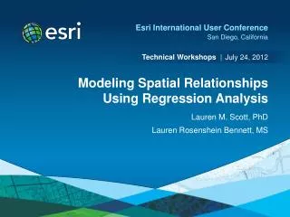
July 2011. Modeling Spatial Relationships using Regression Analysis. Lauren M. Scott, PhD Lauren Rosenshein, MS Mark V. Janikas, PhD. Answering “Why?” Questions. Introduction to Regression Analysis Why are people dying young in South Dakota?. Building a properly specified OLS model

E N D
July 2011 Modeling Spatial Relationships using Regression Analysis Lauren M. Scott, PhD Lauren Rosenshein, MS Mark V. Janikas, PhD
Answering “Why?” Questions • Introduction to Regression Analysis • Why are people dying young in South Dakota? • Building a properly specified OLS model • The 6 things you must check! • Exploring regional variation using GWR Kindly complete a course evaluation: www.esri.com/sessionevals
What can you do with Regression analysis? • Model, examine, and explore spatial relationships • Better understand the factors behind observed spatial patterns • Predict outcomes based on that understanding Geographically Weighted Regression(GWR) Ordinary Least Square (OLS) 100 80 60 40 20 Observed Values Predicted Values 0 20 40 80 100 0 60
What’s the big deal? • Pattern analysis (without regression): • Are there places where people persistently die young? • Where are test scores consistently high? • Where are 911 emergency call hot spots?
What’s the big deal? • Pattern analysis (without regression): • Are there places where people persistently die young? • Where are test scores consistently high? • Where are 911 emergency call hot spots? • Regression analysis: • Why are people persistently dying young? • What factors contribute to consistently high test scores? • Which variables effectively predict 911 emergency call volumes?
Why use regression? • Understand key factors • What are the most important habitatcharacteristics for an endangered bird? • Predict unknown values • How much rainfall will occur in agiven location? • Test hypotheses • “Broken Window” Theory: Is there apositive relationship between vandalism and residential burglary?
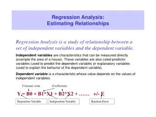
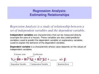
Regression analysis terms and concepts • Dependent variable (Y): What you are trying to model or predict (e.g., residential burglary). • Explanatory variables (X): Variables you believe cause or explain the dependent variable (e.g., income, vandalism, number of households). • Coefficients (β): Values, computed by the regression tool, reflecting the relationship between explanatory variables and the dependent variable. • Residuals (ε): The portion of the dependent variable that isn’t explained by the model; the model under- and over-predictions.
Regression model coefficients • Coefficient sign (+/-) and magnitude reflect each explanatory variable’s relationship to the dependent variable The asterisk * indicates the explanatory variable is statistically significant Intercept 1.625506 INCOME -0.000030 VANDALISM 0.133712 HOUSEHOLDS 0.012425 LOWER CITY 0.136569
OLS Regression Why are people dying young in South Dakota?
OLS analysis Why are people dying young in South Dakota? Do economic factors explain this spatial pattern? Poverty rates explain 66% of the variation in the average age of death dependent variable: Adjusted R-Squared [2]: 0.659 However, significant spatial autocorrelation among model residuals indicates important explanatory variables are missing from the model.
Build a multivariate regression model • Explore variable relationships using the scatterplot matrix • Consult theory and field experts • Look for spatial variables • Run OLS (this is iterative) • Use Exploratory Regression
Our best OLS model • Average Age of Death as a function of: • Poverty Rates • Vehicle Accidents • Lung Cancer • Suicide • Diabetes • This model tells 86% of the story… and the over and under predictions aren’t clustered! But are we done?
Check OLS results 1 Coefficients have the expected sign. 2 No redundancy among explanatory variables. 3 Coefficients are statistically significant. 4 Residuals are normally distributed. 5 Residuals are not spatially autocorrelated. 6 Strong Adjusted R-Square value.
1. Coefficient signs • Coefficients should have the expected signs.
2. Coefficient significance • Look for statistically significant explanatory variables. Robust_Prob 0.000000 * 0.000000 * 0.000011 * 0.000732 * 0.025148 * 0.000692 * Probability 0.000000 * 0.000000 * 0.000000 * 0.000172 * 0.017044 * 0.000134 * * Statistically significant at the 0.05 level Koenker(BP) Statistic [5]: 38.994033 Prob(>chi-squared) (5) degrees of freedom: 0.000626 *
Check for variable redundancy • Multicollinearity: • Term used to describe the phenomenon when two or more of the variables in your model are highly correlated. • Variance inflation factor (VIF): • Detects the severity of multicollinearity. • Explanatory variables with a VIF greater than 7.5 should be removed one by one.
3. Multicollinearity • Find a set of explanatory variables that have low VIF values. • In a strong model, each explanatory variable gets at a different facet of the dependent variable. VIF -------------- 2.351229 1.556498 1.051207 1.400358 3.232363 [1] Large VIF (> 7.5, for example) indicates explanatory variable redundancy.
Checking for model bias • The residuals of a good model should be normally distributed with a mean of zero • The Jarque-Bera test checks model bias
4. Model bias • When the Jarque-Bera test is statistically significant: • The model is biased • Results are not reliable • Often indicates that a key variable is missing from the model [6] Significant p-value indicates residuals deviate from a normal distribution. Jaque-Bera Statistic [6]: 4.207198 Prob(>chi-sq), (2) degrees of freedom: 0.122017
5. Spatial Autocorrelation Statistically significant clustering of under and over predictions. Random spatial pattern of under and over predictions.
6. Model performance • Compare models by looking for the lowest AIC value. • As long as the dependent variable remains fixed, the AIC value for different OLS/GWR models are comparable • Look for a model with a high Adjusted R-Squared value. [2] Measure of model fit/performance. Akaike’s Information Criterion (AIC) [2]: 524.9762 Adjusted R-Squared [2]: 0.8648
Online help is … helpful! The 6 checks: • Coefficients have the expected sign. • Coefficients are statistically significant. • No redundancy among explanatory variables. • Residuals are normally distributed. • Residuals are not spatially autocorrelated. • Strong Adjusted R-Squared value.
Now are we done? • A statistically significant Koenker OLS diagnostic is often evidence that Geographically Weighted Regresion (GWR) will improve model results • GWR allows you to explore geographic variation which can help you tailor effective remediation efforts.
Global vs. local regression models • OLS • Global regression model • One equation, calibrated using data from all features • Relationships are fixed • GWR • Local regression model • One equation for every feature, calibrated using data from nearby features • Relationships are allowed to vary across the study area For each explanatory variable, GWR creates a coefficient surface showing you where relationships are strongest.
GWR Exploring regional variation
Running GWR • GWR is a local spatial regression model • Modeled relationships are allowed to vary • GWR variables are the same as OLS, except: • Do not include spatial regime (dummy) variables • Do not include variables with little value variation
Defining local • GWR constructs an equation for each feature • Coefficients are estimated using nearby feature values • GWR requires a definition for nearby
Defining local • Bandwidth method • AIC or Cross Validation (CV): GWR will find the optimal distance or optimal number of neighbors • Bandwidth parameter: User-provideddistance or user-provided number ofneighbors • GWR requires a definition for nearby • Kernel type • Fixed: Nearby is determined by a fixed distance band • Adaptive: Nearby is determined by a fixed number of neighbors
Interpreting GWR results • Compare GWR R2 and AICc values to OLS R2 and AICc values • The better model has a lower AIC and a high R2. • Model predictions, residuals, standard errors, coefficients, and condition numbers are written to the output feature class.
Mapped Output • Residual maps show model under- and over-predictions. They shouldn’t be clustered. • Coefficient maps show how modeled relationships vary across the study area.
Mapped Output • Maps of Local R2 values show where the model is performing best • To see variation in model stability: apply graduated color rendering to Condition Numbers
GWR prediction Calibrate the GWR model using known values for the dependent variable and all of the explanatory variables. Observed Modeled Predicted Provide a feature class of prediction locations containing values for all of the explanatory variables. GWR will create an output feature class with the computed predictions.
Resources for learning more… • Spatial Pattern Analysis: Mapping Trends and Clusters • Tue 8:30 Rm 2; Wed 3:15 Rm 2 • Modeling Spatial Relationships using Regression Analysis • Tue 10:15 Rm 2; Thu 1:30 Rm 1A/B • Spatial Statistics: Best Practices • Tue 3:15 Rm 2; Thu 3:15 Rm 1A/B • Using R in ArcGIS • Wed 12:00 Rm 1A/B • Road Ahead: Sharing of Analysis (ArcGIS 10.1) • Wed 11:05 Rm 6B
Resources for learning more… QUESTIONS? Kindly complete an evaluation form before you leave • www.esriurl.com/spatialstats • Short videos • Articles and blogs • Online documentation • Supplementary model and script tools • Hot Spot, Regression, and ModelBuilder tutorials LScott@Esri.com LRosenshein@Esri.com