Download
1 / 42
420 likes | 491 Views
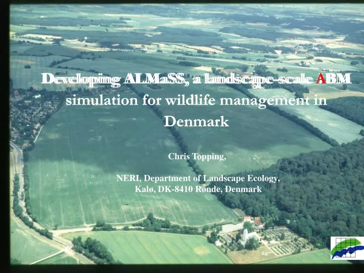
Developing ALMaSS, a landscape-scale IBM simulation for wildlife management in Denmark. Developing ALMaSS, a landscape-scale A BM simulation for wildlife management in Denmark. Chris Topping, NERI , Department of Landscape Ecology, Kalø, DK-8410 Rønde, Denmark.

E N D
Developing ALMaSS, a landscape-scale IBM simulation for wildlife management in Denmark Developing ALMaSS, a landscape-scale ABM simulation for wildlife management in Denmark Chris Topping, NERI, Department of Landscape Ecology, Kalø, DK-8410 Rønde, Denmark
What will the impact on wildlife be of changing to organic farming? Optimal placement of wildlife road tunnels? Conservation Genetics? What happens if we start planting hedgerows or removing hedgerows on a large scale? Will the new motorway have important implications for wildlife? Questions? Population viability? What will the influence of altering pesticide usage be on agricultural wildlife? How can we optimise ground-water protection schemes to maximise wildlife benefit? Fragmentation?
Open field and marginal habitat birds We have adopted an individual-based model approach using indicator species Small mammal herbivore, grassland specialist Large mammal, mosaic specialist Polyphagous predator 1 Large mammal, woodland mosaic specialist Polyphagous predator 2
ALMaSS (Animal, Landscape and Man Simulation System) Animal Models Landscape Model
Field- boundary Road Scrub Field Grass Building Forest River Landscape Structure
Managed by the same farmer Landscape Animation The collection of fields managed forms the farm unit. Each farm is given a type and a crop rotation which it applies to its fields
Spring Barley Crop Management Plan This diagram shows the events leading up to sowing in the spring barley management plan. Start Autumn Plough All events can have time periods, probabilities, dependencies and soil/weather conditions attached. Stock Farmer Arable Farmer Slurry NPK Liquid NH3 PK Manure First the decision is whether to plough in Autumn. Spring Plough If we plough in autumn then the next step is application of fertiliser, otherwise it will depend on whether the farmer is a stock or arable farmer, and what he has available. Harrow Stock Farmer Now if we have not ploughed already, do it in Spring. NPK Next Harrow and if a stock farmer correct the fertiliser using NPK (it is possible to reach here and not to have applied any fertiliser). If he is an arable farmer then fertilise. Sow The red, green and yellow lines show three potential paths through this decision tree. Finally we can sow.
Jan Feb 500 Mar Apr 400 May Jun Jul 300 Aug Vehicles per hour Sep 200 Oct Nov Dec 100 0 00-01 02-03 04-05 06-07 08-09 10-11 12-13 14-15 16-17 18-19 20-21 22-23 Time of day Other Landscape Sub-Models • Seasonal and daily variation in • traffic load on all roads • Soil type, slope and aspect • of all areas • Further subdivision of • forested areas by means • of remote sensing • techniques • Weather data
Types Modelling Population Models IBMs Complexity Gradient Q. Why use the more complex models? • Because we believe they are more accurate at giving answers under certain conditions. In particular when dealing with practical questions, often related to a specific location or structural type of landscape then local interactions between individuals and between individuals and their environments become potentially important.
Agent-based modelling When does an individual becomes an agent? .....When that individual starts to make decisions based on information it gathers, in order to carry out its own agenda (in our case survival and reproduction).
Mate Die Disperse Establish A Territory A transition ? Modelling using states and transitions Exploring Habitat is very low quality
Communication ‘!’ Environmental Conditions Reacting to Events Farming Events Other Organisms +
The results can be used to generate: • Individual-based information - e.g. developmental rates • Spatially related information - e.g. where the animals live, breed or forage • Population information - sum of the individuals to give population descriptors
Some Example Applications • Practical - Environmental Impact Assessment – Pesticides • Ecological – Life-History Strategy Analyses • Theoretical – Population Genetics A selection of results related to agricultural management
Energy Loss Energy Loss Energy Loss Energy Loss Pesticides and Skylarks - The Perceived Wisdom: Assumption: Heterogeneity does not matter
The ALMaSS approach: Using the same basic energetic model, but translating the model to a landscape scale and from a population-based approach to an agent-based one. • Two factors were investigated: • With and Without pesticides • Field Size – 1x & 2x real size
Would we be better off reducing pesticide usage or altering field size conditions? • Pesticides cause a mean of 4% reduction in population size • Large fields cause 37% reduction • There is an interaction between weather and pesticide usage • The interaction is also affected by other factors (time-lags & other mortalities) (Topping & Odderskær in prep)
Analyses of life-history strategies • For example: Polyphagous predator studies • How do LHSs interact with man’s management of the landscape? • Differential sensitivity to pesticides • How do LHSs interact with landscapes? • We know some species do particularly well in agricultural landscapes. This probably has something to do with their LHS – can we quantify this?
Damaging time to spray Safer time to spray Dispersal Uncertain Effects Here the effect depends upon the area and timing of pesticides. the more synchronised in time and space the worse the impact. Minimising Pesticide Impacts How does area and timing of pesticide applications effect the dynamics of non-target organisms?
By altering life-history parameters we can simulate a range of different species:
The ratio a/b is smaller in small fields indicating an interaction between field size and movement - lower movement rate has a smaller penalty in small fields a b a b Smaller populations in large fields General increase in population size with more field boundaries Steep increase in population size with increasing movement rate Simulations of carabid movement rates, proportion of fields with grassy boundaries and field size
SOURCE DF SS F-ratio P field size 1 12.1 161.0 < 0.0001 dispersal ability 3 9282.6 41529.5 < 0.0001 boundary condition 2 44.1 292.6 < 0.0001 field × dispersal 3 6.9 30.5 < 0.0001 field × boundary 2 1.0 6.8 0.0011 dispersal × boundary 6 36.8 81.4 < 0.0001 time 1 0.4 5.7 0.0168 run 4 0.3 1.0 0.4188 (Bilde & Topping in prep)
Population Genetics Important because it can show past population events, current population structure and predict future population viability
a c a d b b a c a a d a b a d c c a a a d b c a a b a b a a a a Genetic Modelling in ALMaSS This is made possible by the fact that we can track matings between individuals, therefore we can track gene-flow. The prototype for this is the field vole model. Model field voles have a simple genetic code which is made up of a single chromosome, with 16 loci, and four alleles at each locus. Each chromosome is made of two strands of DNA, therefore each vole carries 32 alleles in 16 pairs e.g.
+ The combination of the agent-based model and genetics opens the way for a range of interesting questions. • For example: • Investigating fragmentation effects • Population viability and the risk of extinction vortices • But there is the even more tantalizing possibility of linking the genotype with the phenotype (in this case the model parameters). • Evolution of dispersal • Optimal life-history strategies • Theoretical genetics e.g. creation of hybrid zones
Implications of annual local population perturbations on the genetic diversity of voles The population perturbation produced a reduction of 0.8% of the landscape carrying capacity measured by N. But..a reduction of 24.6% inexpected heterozygosity (He ). This indicates a change of the genetic structure of the population due to the fragmentation of the landscape by the perturbation.
Main Contributors to ALMaSS: Chris Topping Peter Odderskær Jane Uhd Jepsen Frank Nikolajsen Cino Pertoldi Peter Lange Poul Nygaard Andersen Geoff Groom Trine Bilde Pernille Thorbek Siri Østergaard Tine Sussi Hansen
Practical Session • In 2 parts: • Some technical information about the building of ALMaSS • - What kinds of things do we have to deal with technically - some examples of landcape and animal modelling. • Hands on use of a simulation
Technical Information: • Model is programmed in C++ - an object-oriented language with good code re-use features and very efficient execution code. • When running the basic model will occupy a lot of RAM. A typical 10 x 10km simulation between 1 and 1.5 GB RAM, but some require 2.0 GB • Simulation runs can last up to two weeks for numerous species with complex behaviours
1) Mapping Landscape Modelling: 1) Mapping • All available electronic data sources are utilised, together with aerial photos and ground truthing • Data is initially collected together in a GIS where the structure and habitat information can be combined. • The GIS exports a raster map together with a polygon reference. The raster map is then used to represent the landscape in the computer – a technique called ’fly-weight’ is used to maximise computation efficiency.
If each polygon is described using 10 pieces of information 9 x 9 x 10 = 810 pieces of info. 12 x 10 = 120 pieces of info. 1 2 3 4 5 6 7 8 One copy of the information for each polygon 9 10 11 12 Fly-weight (Gamma et al, 1994) Uses sharing to support large numbers of objects efficiently
Female Skylark Behavioural Diagram Immigration Emigrating Floating Arrive In Sim. Area Flocking Finding Territory Attract Mate Die Building Up resources Initiation Temp. Leave Area Give Up Territory Follow Mate Care for Young Stopping Breeding Prepare For Breeding New Brood Egg Hatch Incubating Lay Eggs Make Nest
Calculate food accessibility for each habitat Use time to feed Adult Foraging • Calculate the area of each habitat polygon in home range • Interrogate the polygon for the insect biomass • Determine the total available resource by multiplication Assess home range for insect resources • Using a matrix based on the weather, vegetation height and biomass, calculate the feeding hindrance factor for each habitat polygon • Based on the resource present an accessibility allocate the feeding time available to maximise the insect resource collected, or calculate the time required to obtain a target amount of resource
Egg Development Development is a function of temperature experienced by the eggs. This in turn is related to the environmental temperature, and the time the female spends incubating. • Get the time required for the female to feed herself (get enough food to maintain her EM . • Assume that the time is spent evenly through the day so that 20% of the day feeding is assumed to be 20% of each hour therefore 12 mins off the nest in each hour. • The cooling effect can then be calculated using the ambient temperature and a cooling rate for skylark sized eggs. • It is assumed that the cooling rate and warming rate are identical, so the time spent cooling is the time spent to raise the egg to the females body temperature. • The day degrees experienced by the egg are therefore twice the time spent off the nest multiplied by the mean cooling/warming temperature, plus the rest of time at incubating temperature. • Egg mortality can result if the female spends too long from the nest. data sources: Kendeigh et al., Avian Energetics & O’Conner 1985 The growth and development of birds
Nestling Growth Each day each parent feed insects to the young after they have obtained enough to cover their own EM. They are fed preferentially based on the size of the young, if two or more are equal sized then food allocation is random. Growth is given by: (Insects Ingested * Insect Assimilation Rate * Conversion EfficiencyAGE) - EM Data source Pinowski & Kendeigh Granivorous Birds in Ecosystems
Putting this together with field data: • There is one main factor that we have to base our energetics on. This is the extraction efficiency of the skylarks. • The problem is this cannot be measured. • However, by treating it as a fitting parameter it is possible to vary this figure and evaluate the result. • By altering extraction efficiency it was possible to iterate to a value which resulted in simulated hatching and development rates being equal to those observed in the field: