Download
1 / 47
470 likes | 565 Views
Explore combinatorial search methods in this course, with assignments and exam details included. Don't miss essential information about assignments and exercise sessions.

E N D
Combinatorial Search Spring 2008 (Fourth Quarter)
Some practical remarks • Homepage: www.daimi.au.dk/dKS • Exam: Oral, 7-scale 30 minutes, including overhead, no preparation. • There will be three compulsory assignments. If you want to transfer credit from last year, let me know as soon as possible and before May 1. • The solution to the compulsory assignments should be handed in at specific exercise sessions and given to the instructor in person. • Text: “Kompendium” available at GAD + online notes.
Exercise classes • You can switch classes iff you find someone to switch with. • To find someone, post an add in the group dSoegOpt … Or try finding someone after the class! • Exercise classes are on specific dates, see webpage
Frequently asked questions about compulsory assignments • Q: Do I really have to hand in all three assignments? • A:YES! • Q: Do I really have to hand in all three assignments on time? • A:YES! • Q: What if I can’t figure out how to solve them? • A:Ask your instructor. Start solving them early, so that you will have sufficient time. • Q: What if I get sick or my girlfriend breaks up or my hamster dies? • A: Start solving them early, so that you will have sufficient time in case of emergencies. • Q: Do I really have to hand in all three assignments? • A:YES!
“Optimization” – a summary! Mixed Integer Linear Programming Exponential By Branching … TSP … Efficient by Local Search ? Linear Programming Min Cost Flow = reduction Max Flow Maximum matching Shortest paths
NP-completeness Mixed Integer Linear Programming Exponential By Branching … TSP … Efficient by Local Search ? Linear Programming Min Cost Flow = reduction Max Flow Maximum matching Shortest paths
NP-completeness Mixed Integer Linear Programming … TSP Exponential No reduction, unless P=NP Efficient by Local Search Linear Programming Min Cost Flow = reduction Max Flow Maximum matching Shortest paths
Problems: Languages • A languageL is a subset of {0,1}*. • A language models a decision problem: Members of L are the yes-instances, non-members are the no-instances. • This is the only kind of problem our theory shall be concerned with!
Restriction: Inputs Boolean Strings • Strings over an arbitrary alphabet can be represented as Boolean Strings (Ex: ascii, unicode). • In reality, computers may only hold Boolean strings (their memory image is a bit string). • Arbitrary real numbers may not be represented but this is intentional!
Models of Computation • Model 1: Our computer holds exact real numbers. The size of the input is the number of real numbers in the input. The time complexity of an algorithm is the number of arithmetic operations performed. • Model 2: Our computer holds bits and bytes. The size of the input is the number of bits in the input. The time complexity of an algorithm is the number of bit-operations performed. • We know an efficient algorithm for linear programming in Model 2 but not model 1. • The NP-completeness theory is intended to capture Model 2 and not Model 1.
How to encode max flow instance? java MaxFlow 6#0|16|13|0|0|0#0|0|10|12|0|0 #0|4|0|0|14|0#0|0|9|0|0|20 #0|0|0|7|0|4|#0|0|0|0|0|0
Restriction: All inputs “legal”. • Any string should be either a yes-string or a no-string. • It would be nice to also have “malformed” strings. • However, we shall just lump the malformed strings with the no-strings.
Restriction:Output yes or no • Suppose we want to consider computing a function, f: {0,1}* ! {0,1}*. • Stand-in for f: Lf= {<x, b(j), y> | f(x)j = y} • Lf has an efficient algorithm if and only if f has an efficient algorithm.
Restriction: functions • OPT: Given description of F, f find x2F maximizing f(x). • There may be several optimal solutions. OPT does not seem to be captured easily by a function. • Stand-in for OPT: LOPT = { < desc(F), desc(f), b(), b() > | some x2F has f(x) ¸ / }
LOPT vs. OPT • LOPT may be easy to solve even though OPT is hard to solve, so LOPT is not a perfect stand-in. • However, if LOPT has no efficient solution, then OPT has no efficient solution, so LOPT can still be used to argue that OPT is hard.
Turing Machines • A Turing machine consists of an infinite tape, divided into cells, each holding a symbol from alphabet that includes 0,1,#. • A tape head is at any point in time positioned at a cell. • A finite control reads the symbol at the head, updates the symbol at the head and the position of the head.
Finite Control • Finite set of states Q. The control is in exactly one of the state. Three special states: start, accept, reject. • Transition function:
Running the machine on an input • The input string is placed on the tape (surrounded by blanks) and the head positioned to the immediate left of the input. The initial state of the finite control is start. • If the finite control eventually goes to accept state, the input is accepted (“the machine outputs yes”). • If the finite control eventually goes to reject state, the input is rejected (“the machine outputs no”). • The machine is said to decide a language L if it accepts all members of L and rejects all members of {0,1}*-L.
Some Turing Machine Applets http://math.hws.edu/TMCM/java/labs/xTuringMachineLab.html http://www.igs.net/~tril/tm/tm.html http://web.bvu.edu/faculty/schweller/Turing/Turing.html
If you want to make rigorous the notion of an “efficient algorithm” why do you choose such a hopelessly inefficient device ??!?
Church-Turing Thesis Any decision problem that can be solved by some mechanical procedure, can be solved by a Turing machine.
Polynomial Church-Turing thesis A decision problem can be solved in polynomial time by using a reasonable sequential model of computation if and only if it can be solved in polynomial time by a Turing machine.
The complexity class P • P := the class of decision problems (languages) decided by a Turing machine so that for some polynomial p and all x, the machine terminates after at most p(|x|) steps on input x. • By the Polynomial Church-Turing Thesis, P is “robust” with respect to changes of the machine model. • Is P also robust with respect to changes of the representation of decision problems as languages?
How to encode max flow instance? java MaxFlow 6#0|16|13|0|0|0#0|0|10|12|0|0 #0|4|0|0|14|0#0|0|9|0|0|20 #0|0|0|7|0|4|#0|0|0|0|0|0
java MaxFlow 111111 #|1111111111111111|1111111111111||| #||1111111111|111111111111|| #|1111|||11111111111111| #||111111111|||11111111111111111111 #|||1111111||1111 #|||||
Polynomial time computable maps f: {0,1}* ! {0,1}* is called polynomial time computable if for some polynomial p, - For all x, |f(x)| ·p(|x|). - Lf2P.
Polynomially equivalent representations • A representation of objects (say graphs, numbers) as strings is good if the language of valid representations is in P. • Two different representations of objects are called polynomially equivalent if we may translate between them using polynomial time computable maps. • Ex: Adjacency matrices vs. Edge lists • Ex: Binary vs. Decimal • Counterexample: Binary vs. Unary
Robustness of Representation • Given two good, polynomially equivalent representations of the instances of a decision problem, resulting in languages L1 and L2 we have L12P iff L22P.
Search Problems: NP • We want to capture decision problems that can be solved by exhaustive search of the following kind. • Go through a space of possible solutions, checking for each one of them if it is an actual solutions (in which case the answer is yes). • Example: Compositeness. Given a number in binary, is it a product of smaller numbers?
Search Problems: NP L is in NP iff there is a language L’ in P and a polynomial p so that:
Intuition • The y-strings are the possible solutions to the instance x. • We require that solutions are not too long and that it can be checked efficiently if a given y is indeed a solution (we have a “simple” search problem)
P vs. NP • P is a subset of NP • Is P=NP? Then any “simple” search problem has a polynomial time algorithm. • This is the most famous open problem of mathematical computer science!
P vs. NP and mathematics • If P=NP, mathematicians may be replaced by (much more reliable) computers: P=NP ) There is an algorithmic procedure that takes as input any formal math statement and always outputs its shortest formal proof in time polynomial in the length of the proof. • This is usually regarded (in particular by mathematicians!) as evidence that P and NP are different.
Reductions • A reduction r of L1 to L2 is a polynomial time computable map so that 8 x: x 2 L1 iff r(x) 2L2 • We write L1· L2 if L1 reduces to L2. • Intuition: Efficient software for L2 can also be used to efficiently solve L1.
Properties of reductions Transitivity: L1·L2Æ L2· L3)L1·L3 Downward closure of P: L1·L2Æ L22P ) L12P. • Follows from Polynomial Church-Turing thesis.
NP-hardness • A language L is called NP-hard iff 8L’ 2NP: L’ ·L • Intuition: Software for L is strong enough to be used to solve any simple search problem. • Proposition: If some NP-hard language is in P, then P=NP.
NPC • A language L 2NP that is NP-hard is called NP-complete. • NPC := the class of NP-complete problems. • Proposition: L2NPC) [L2P iff P=NP].