Download
1 / 37
390 likes | 587 Views
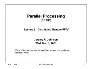
Parallel Processing (CS 730) Lecture 9: Distributed Memory FFTs *. Jeremy R. Johnson Wed. Mar. 1, 2001 *Parts of this lecture was derived from material from Johnson, Johnson, Pryor. Introduction.

E N D
Parallel Processing (CS 730)Lecture 9: Distributed Memory FFTs* Jeremy R. Johnson Wed. Mar. 1, 2001 *Parts of this lecture was derived from material from Johnson, Johnson, Pryor. Parallel Processing
Introduction • Objective: To derive and implement a distributed-memory parallel program for computing the fast Fourier transform (FFT). • Topics • Derivation of the FFT • Iterative version • Pease Algorithm & Generalizations • Tensor permutations • Distributed implementation of tensor permutations • stride permutation • bit reversal • Distributed FFT Parallel Processing
FFT as a Matrix Factorization Compute y = Fnx, where Fnis n-point Fourier matrix. Parallel Processing
Matrix Factorizations and Algorithms function y = fft(x) n = length(x) if n == 1 y = x else % [x0 x1] = L^n_2 x x0 = x(1:2:n-1); x1 = x(2:2:n); % [t0 t1] = (I_2 tensor F_m)[x0 x1] t0 = fft(x0); t1 = fft(x1); % w = W_m(omega_n) w = exp((2*pi*i/n)*(0:n/2-1)); % y = [y0 y1] = (F_2 tensor I_m) T^n_m [t0 t1] y0 = t0 + w.*t1; y1 = t0 - w.*t1; y = [y0 y1] end Parallel Processing
Rewrite Rules Parallel Processing
FFT Variants • Cooley-Tukey • Recursive FFT • Iterative FFT • Vector FFT (Stockham) • Vector FFT (Korn-Lambiotte) • Parallel FFT (Pease) Parallel Processing
Example TPL Programs ; Recursive 8-point FFT (compose (tensor (F 2) (I 4)) (T 8 4) (tensor (I 2) (compose (tensor (F 2) (I 2)) (T 4 2) (tensor (I 2) (F 2)) (L 4 2)) (L 8 2)) ; Iterative 8-point FFT (compose (tensor (F 2) (I 4)) (T 8 4) (tensor (I 2) (F 2) (I 2)) (tensor (I 2) (T 4 2)) (tensor (F 2) (I 4)) (tensor (I 2) (L 4 2) (L 8 2)) Parallel Processing
FFT Dataflow • Different formulas for the FFT have different dataflow (memory access patterns). • The dataflow in a class of FFT algorithms can be described by a sequence of permutations. • An “FFT dataflow” is a sequence of permutations that can be modified with the insertion of butterfly computations (with appropriate twiddle factors) to form a factorization of the Fourier matrix. • FFT dataflows can be classified wrt to cost, and used to find “good” FFT implementations. Parallel Processing
Distributed FFT Algorithm • Experiment with different dataflow and locality properties by changing radix and permutations Parallel Processing
Cooley-Tukey Dataflow Parallel Processing
Pease Dataflow Parallel Processing
Tensor Permutations • A natural class of permutations compatible with the FFT. Let be a permutation of {1,…,t} • Mixed-radix counting permutation of vector indices • Well-known examples are stride permutations and bit-reversal. Parallel Processing
Example (Stride Permutation) • 000 000 • 001 100 • 010 001 • 011 011 • 100 010 • 101 110 • 110 101 • 111 111 Parallel Processing
Example (Bit Reversal) • 000 000 • 001 100 • 010 010 • 011 110 • 100 001 • 101 101 • 110 011 • 111 111 Parallel Processing
Twiddle Factor Matrix • Diagonal matrix containing roots of unity • Generalized Twiddle (compatible with tensor permutations) Parallel Processing
pid offset bk+l-1 ……blbl-1 …...……... b1 b0 Distributed Computation • Allocate equal-sized segments of vector to each processor, and index distributed vector with pid and local offset. • Interpret tensor product operations with this addressing scheme Parallel Processing
Distributed Tensor Product and Twiddle Factors • Assume P processors • InA, becomes parallel do over all processors when n P. • Twiddle factors determined independently from pid and offset. Necessary bits determined from I, J, and (n1,…,nt) in generalized twiddle notation. Parallel Processing
pid offset bk+l-1 ……blbl-1 …...……... b1 b0 b(k+l-1) … b(l) b(l-1) ………... b(1)b(0) Distributed Tensor Permutations Parallel Processing
Classes of Distributed Tensor Permutations • Local (pid is fixed by ) Only permute elements locally within each processor • Global (offset is fixed by ) Permute the entire local arrays amongst the processors • Global*Local (bits in pid and bits in offset moved by , but no bits cross the pid/offset boundary) Permute elements locally followed by a Global permutation • Mixed (at least one offset and pid bit are exchanged) Elements from a processor are sent/received to/from more than one processor Parallel Processing
000|**0 000|0** 000|**1 100|0** 001|**0 000|1** 001|**1 100|1** 010|**0 001|0** 010|**1 101|0** 011|**0 001|1** 011|**1 101|1** 100|**0 010|0** 100|**1 110|0** 101|**0 010|1** 101|**1 110|1** 110|**0 011|0** 110|**1 111|0** 111|**0 011|1** 111|**1 111|1** Distributed Stride Permutation Parallel Processing
1 0 Y(4:1:3) 2 X(1:2:7) 7 X(0:2:6) Y(0:1:7) 3 6 4 5 Communication Pattern Parallel Processing
6 6 1 1 2 2 3 3 5 5 7 7 0 0 4 4 Communication Pattern Each PE sends 1/2 data to 2 different PEs Parallel Processing
6 6 1 1 2 2 3 3 5 5 7 7 0 0 4 4 Communication Pattern Each PE sends 1/4 data to 4 different PEs Parallel Processing
6 6 1 1 2 2 3 3 5 5 7 7 0 0 4 4 Communication Pattern Each PE sends1/8 data to 8 different PEs Parallel Processing
Implementation of Distributed Stride Permutation D_Stride(Y,N,t,P,k,M,l,S,j,X) // Compute Y = L^N_S X // Inputs // Y,X distributed vectors of size N = 2^t, // with M = 2^l elements per processor // P = 2^k = number of processors // S = 2^j, 0 <= j <= k, is the stride. // Output // Y = L^N_S X p = pid for i=0,...,2j-1 do put x(i:S:i+S*(n/S-1)) in y((n/S)*(p mod S):(n/S)*(p mod S)+N/S-1) on PE p/2^j + i*2^{k-j} Parallel Processing
6 6 1 1 2 2 3 3 5 5 7 7 0 0 4 4 Cyclic Scheduling Each PE sends 1/4 data to 4 different PEs Parallel Processing
Distributed Bit Reversal Permutation • Mixed tensor permutation • Implement using factorization b7b6b5 b4b3b2b1b0 b0b1b2 b3b4b5b6b7 b7b6b5 b4b3b2b1b0 b5b6b7 b0b1b2b3b4 Parallel Processing
Experiments on the CRAY T3E • All experiments were performed on a 240 node (8x4x8 with partial plane) T3E using 128 processors (300 MHz) with 128MB memory • Task 1(pairwise communication) Implemented with shmem_get, shmem_put, and mpi_sendrecv • Task 2 (all 7! = 5040 global tensor permutations) Implemented with shmem_get, shmem_put, and mpi_sendrecv • Task 3 (local tensor permutations of the form I L I on vectors of size 2^22 words - only run on a single node) Implemented using streams on/off, cache bypass • Task 4 (distributed stride permutations) Implemented using shmem_iput, shmem_iget, and mpi_sendrecv Parallel Processing
Task 1 Performance Data Parallel Processing
Task 2 Performance Data Parallel Processing
Task 3 Performance Data Parallel Processing
Task 4 Performance Data Parallel Processing
Network Simulator • An idealized simulator for the T3E was developed (with C. Grassl from Cray research) in order to study contention • Specify processor layout and route table and number of virual processors with a given start node • Each processor can simultaneously issue a single send • Contention is measured as the maximum number of messages across any edge/node • Simulator used to study global and mixed tensor permutations. Parallel Processing
Task 2 Grid Simulation Analysis Parallel Processing
Task 2 Grid Simulation Analysis Parallel Processing
Task 2 Torus Simulation Analysis Parallel Processing
Task 2 Torus Simulation Analysis Parallel Processing