Download
1 / 39
670 likes | 1.73k Views
Costs, Isocost and Isoquant. Outline. Costs In The Short Run Allocating Production Between Two Processes The Relationship Among MP, AP, MC, And AVC Costs In The Long Run Long-run Costs And The Structure Of Industry The Relationship Between Long-run And Short-run Cost Curves. 10- 2.

E N D
Outline • Costs In The Short Run • Allocating Production Between Two Processes • The Relationship Among MP, AP, MC, And AVC • Costs In The Long Run • Long-run Costs And The Structure Of Industry • The Relationship Between Long-run And Short-run Cost Curves 10-2
Costs In The Short Run • Fixed cost (FC):cost that does not vary with the level of output in the short run (the cost of all fixed factors of production). • Variable cost (VC):cost that varies with the level of output in the short run (the cost of all variable factors of production). • Total cost (TC):all costs of production: the sum of variable cost and fixed cost. 10-3
Figure 10.3: The Production Function Q = 3KL, with K = 4 10-6
Figure 10.4: The Total, Variable, and Fixed Cost Curves for the Production Function Q-3KL 10-7
Costs In The Short Run • Average fixed cost (AFC):fixed cost divided by the quantity of output. • Average variable cost (AVC):variable cost divided by the quantity of output. • Average total cost (ATC):total cost divided by the quantity of output. • Marginal cost (MC):change in total cost that results from a 1-unit change in output. 10-8
Graphing The Short-run Average AndMarginal Cost Curves • Geometrically, average variable cost at any level of output Q may be interpreted as the slope of a ray to the variable cost curve at Q. 10-9
Figure 10.5: The Marginal, Average Total, Average Variable, and Average Fixed Cost Curves 10-10
Figure 10.6: Quantity vs. Average Costs ATC-AVC=AFC 10-11
Marginal Costs • is the same as the cost of expanding output (or the savings from contracting). • the most important of the seven cost curves. • Geometrically, at any level of output may be interpreted as the slope of the total cost curve at that level of output. MC=ΔTC/ ΔQ 10-12
Marginal and Average Costs • When Marginal Cost is less than average cost (either ATC or AVC), the average cost curve must be decreasing with output; and when MC is greater than average cost, average cost must be increasing with output. 10-13
Figure 10.7: Cost Curves for a Specific Production Process MC=ΔTC/ ΔQ=AVC Constant marginal cost, and average variable cost 10-14
The Cost-minimizing condition: Allocating Production BetweenTwo Processes • Let QTbe the total amount to be produced, and let Q1 and Q2 be the amounts produced in the first and second processes (as in the fish boat example in chapter 9). And suppose the marginal cost in one process at very low levels of output is lower than the marginal cost at QTunits of output in the other (which ensures that both processes will be used). • The values of Q1and Q2that solve this problem will then be the ones that result in equal marginal costs for the two processes. • The lower the marginal cost, the higher the profit. (recall the profit maximizing condition) 10-15
Figure 10.8: The Minimum Cost Production Allocation The minimum-cost condition is that with QA +QB=32. Equating marginal costs, we have 10-16
Figure 10.9: The Relationship Between MP, AP, MC, and AVC 10-17
Costs In The Long Run • Isocost line:a set of input bundles each of which costs the same amount. • To find the minimun cost point we begin with a specific isoquant then superimpose a map of isocost lines, each corresponding to a different cost level. The least-cost input bundle corresponds to the point of tangency between an isocost line and the specified isoquant. 10-18
Figure 10.13: Different Waysof Producing 1 Ton of Gravel Note: higher capital input in US than in Nepal (labor intensive) 10-20
Figure 10.11: The Maximum Outputfor a Given Expenditure Profit maximizing condition: marginal product of 1 krona invested in capital equals to marginal product of labor. 10-21
Figure 10.12: The Minimum Costfor a Given Level of Output Optimal point is the minimum cost given output level. At the tangency, the slopes of both Isocost and isoquant are the same: -w/r MRTS = MPL/MPK = w/r 10-22
Profit maximizing condition • Note, when the equilibrium is breached, one should invest in the inputs that give higher marginal product per unit of investment.
Figure 10.14: The Effect of a Minimum Wage Law on Unemployment of Skilled Labor To the extent skilled workers are substitutes to unskilled workers, minimum wage will benefit the skilled workers. w 10-24
The Relationship Between Optimal Input ChoiceAnd Long-run Costs • Output expansion path:the locus of tangencies (minimumcost input combinations) traced out by an isocost line of given slope as it shifts outward into the isoquant map for a production process. (see graph next) 10-25
Figure 10.16: The Long-Run Total, Average, and Marginal Cost Curves 10-27
The Relationship Between Optimal Input Choice And Long-run Costs • Constant returns to scale - long-run total costs are exactly proportional to output. • Decreasing returns to scale - a given proportional increase in output requires a greater proportional increase in all inputs and hence a greater proportional increase in costs. • Increasing returns to scale - long-run total cost rises less than in proportion to increases in output. 10-28
Figure 10.17: The LTC, LMC and LAC Curves with Constant Returns to Scale Long run marginal and long run average cost costant under the constant return to scale production (constant cost industry) 10-29
Figure 10.18: The LTC, LAC and LMC Curves for a Production Process with Decreasing Returns to Scale Long run marginal and long run average cost increasing under the decreasing return to scale production! 10-30
Figure 10.19: The LTC, LAC and LMC Curves for a Production Process with Increasing Returns to Scale Long run marginal and long run average cost decreasing under the increasing return to scale production! 10-31
Long-run Costs And The StructureOf Industry • Natural monopoly:an industry whose market output is produced at the lowest cost when production is concentrated in the hands of a single firm. (Efficient scale covers all the demand.) • Minimum efficient scale: the level of production required for LAC to reach its minimum level. 10-32
Figure 10.20: LAC Curves Characteristic of Highly Concentrated Industrial Structures 10-33
Figure 10.21: LAC Curves Characteristic of Unconcentrated Industry Structures 10-34
Figure 10.22: The Family of Cost Curves Associated with a U-Shaped LAC Note as capital increases, the LAC reaches a minimum level, which is the minimum efficient scale of production. 10-35
Figure A10.1: The Short-run and Long-Run Expansion Paths Note: In the short run, the real capital is fixed. 10-36
Figure A10.2: The LTC and STC Curves Associated with the Isoquant Map in Figure A.10.1 10-37
CONSTANT-COST INDUSTRY • A perfectly competitive industry with a horizontal long-run industry supply curve that results because expansion of the industry causes no change in production cost or resource prices. • A constant-cost industry occurs because the entry of new firms, prompted by an increase in demand, does not affect the long-run average cost curve of individual firms. In equilibrium, LAC=LMC=P • See graph next.
Figure A10.3: The LAC, LMC, and Two ATC Curves Associated with the Cost Curves from Figure A.10.2 constant-cost industry 10-39