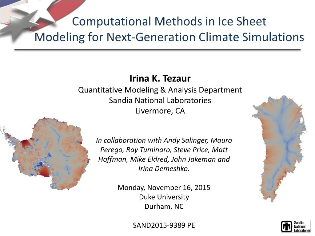
Computational Methods in Ice Sheet Modeling for Next-Generation Climate Simulations

1. Computational Methods in Ice Sheet Modeling for Next-Generation Climate Simulations Irina K. Tezaur Quantitative Modeling & Analysis Department Sandia National Laboratories Livermore, CA In collaboration with Andy Salinger, Mauro Perego, Ray Tuminaro, Steve Price, Matt Hoffman, Mike Eldred, John Jakeman and Irina Demeshko. Monday, November 16, 2015 Duke University Durham, NC SAND2015-9389 PE

2. Outline • Motivation. • The PISCEES project. • The Ice Sheet Equations. • The Albany/FELIX Steady Stress-Velocity Solver. • Deterministic Inversion for Ice Sheet Initialization. • Dynamic Simulations of Ice Sheet Evolution. • Uncertainty Quantification. • Summary & future work.

3. Outline • Motivation. • The PISCEES project. • The Ice Sheet Equations. • The Albany/FELIX Steady Stress-Velocity Solver. • Deterministic Inversion for Ice Sheet Initialization. • Dynamic Simulations of Ice Sheet Evolution. • Uncertainty Quantification. • Summary & future work.

4. Motivation Sea-level rise has received a lot of media attention in recent years! • Full deglaciation: sea level could rise up to ~65 meters* • Potential contributions to sea level rise by ice sheet: • Greenland ice sheet: ~7 meters • East Antarctic ice sheet: ~53 meters • West Antarctic ice sheet: ~5 meters *Estimates given by Prof. Richard Alley of Penn State who testified in 1999 about climate change to Al Gore.

5. Motivation Sea-level rise has received a lot of media attention in recent years! • 2012 Award Winning Film “Chasing Ice”: National Geographic photographer James Balogdeploys time-lapse cameras to capture a multi-year record of the world's changing glaciers.

6. Motivation Sea-level rise has received a lot of media attention in recent years! • 2015 Headlines: “Former Top NASA Scientist Predicts Catastrophic Rise in Sea Levels”, “Earth’s Most Famous Climate Scientist Issues Bombshell Sea Level Warning”, “Climate Seer James Hansen Issues His Direst Forecast Yet” ?

7. Motivation Mass loss from the Greenland & Antarctic ice sheets is accelerating!

8. Earth System Models (ESMs) Ice sheets are part of a global climate system. Mass balance: change in ice sheet mass = mass in – mass out sea level change snow fall melt,calving

9. Earth System Models: CESM, DOE-ESM • An ESM has six modular components: • Atmosphere model • Ocean model • Sea ice model • Land ice model • Land model • Flux coupler Land Surface (ice sheet surface mass balance) Ice Sheet (dynamics) Atmosphere Ocean Flux Coupler Sea Ice Goal of ESM: to provide actionable scientific predictions of 21st century sea-level rise (including uncertainty). • Land Ice Model passes: • Elevation • Revised land ice distribution • Oceanic heat and moisture fluxes (icebergs) • Revised sub-shelf geometry • Climate Model passes: • Surface mass balance (SMB) • Boundary temperatures • Sub-shelf melting

10. Earth System Models: CESM, DOE-ESM • An ESM has six modular components: • Atmosphere model • Ocean model • Sea ice model • Land ice model • Land model • Flux coupler Land Surface (ice sheet surface mass balance) Ice Sheet (dynamics) Atmosphere Ocean Flux Coupler Sea Ice 2012: No robust land ice model!  Goal of ESM: to provide actionable scientific predictions of 21st century sea-level rise (including uncertainty). • Land Ice Model passes: • Elevation • Revised land ice distribution • Oceanic heat and moisture fluxes (icebergs) • Revised sub-shelf geometry • Climate Model passes: • Surface mass balance (SMB) • Boundary temperatures • Sub-shelf melting

11. Outline • Motivation. • The PISCEES project. • The Ice Sheet Equations. • The Albany/FELIX Steady Stress-Velocity Solver. • Deterministic Inversion for Ice Sheet Initialization. • Dynamic Simulations of Ice Sheet Evolution. • Uncertainty Quantification. • Summary & future work.

12. The PISCEES Project • In its fourth assessment report (AR4)* in 2007, the Intergovernmental Panel on Climate Change (IPCC) declined to include estimates of future sea-level rise from ice sheet dynamics due to the inability of ice sheet models to mimic or explain observed dynamic behaviors, e.g., the acceleration and thinning then occurring on several of Greenland’s large outlet glaciers. * Solomon, S., Qin, D., Manning, M., Chen, Z., Marquis, M., Averyt, K., Tignor, M., and Miller, H. “Climate change 2007: The physical science basis, Contribution of Working Group I to the Fourth Assessment Report of the Intergovernmental Panel on Climate Change”, Cambridge Univ. Press, Cambridge, UK, 2007.

13. The PISCEES Project • In its fourth assessment report (AR4)* in 2007, the Intergovernmental Panel on Climate Change (IPCC) declined to include estimates of future sea-level rise from ice sheet dynamics due to the inability of ice sheet models to mimic or explain observed dynamic behaviors, e.g., the acceleration and thinning then occurring on several of Greenland’s large outlet glaciers. • Although ice sheet models have improved in recent years, much work is needed to make these models robust and efficient on continental scales and to quantify uncertainties in their projected outputs. * Solomon, S., Qin, D., Manning, M., Chen, Z., Marquis, M., Averyt, K., Tignor, M., and Miller, H. “Climate change 2007: The physical science basis, Contribution of Working Group I to the Fourth Assessment Report of the Intergovernmental Panel on Climate Change”, Cambridge Univ. Press, Cambridge, UK, 2007.

14. The PISCEES Project • In its fourth assessment report (AR4)* in 2007, the Intergovernmental Panel on Climate Change (IPCC) declined to include estimates of future sea-level rise from ice sheet dynamics due to the inability of ice sheet models to mimic or explain observed dynamic behaviors, e.g., the acceleration and thinning then occurring on several of Greenland’s large outlet glaciers. • Although ice sheet models have improved in recent years, much work is needed to make these models robust and efficient on continental scales and to quantify uncertainties in their projected outputs. PISCEES (Predicting Ice Sheet Climate & Evolution at Extreme Scales) aims to: Develop/apply robust, accurate, scalable dynamical cores (dycores) for ice sheet modeling on structured and unstructured meshes. Evaluate models using new tools and data sets for verification/validation and uncertainty quantification. Integrate models/tools into DOE-supported Earth System Models. * Solomon, S., Qin, D., Manning, M., Chen, Z., Marquis, M., Averyt, K., Tignor, M., and Miller, H. “Climate change 2007: The physical science basis, Contribution of Working Group I to the Fourth Assessment Report of the Intergovernmental Panel on Climate Change”, Cambridge Univ. Press, Cambridge, UK, 2007.

15. The PISCEES Project (cont’d) FSU FELIX FSU Finite Element Full Stokes Model PISCEES SciDAC Application Partnership (DOE’s BER + ASCR divisions) Start date: June 2012 5 years 3 land-ice dycores developed under PISCEES Albany/FELIX SNL Finite Element “First Order” Stokes Model Increased fidelity BISICLES LBNL Finite Volume L1L2 Model PISCEES: Predicting Ice Sheet Climate & Evolution at Extreme Scales FELIX:Finite Elements for Land Ice eXperiments BISICLES: Berkeley Ice Sheet Initiative for Climate at Extreme Scales

16. The PISCEES Project (cont’d) FSU FELIX FSU Finite Element Full Stokes Model PISCEES SciDAC Application Partnership (DOE’s BER + ASCR divisions) Start date: June 2012 5 years 3 land-ice dycores developed under PISCEES Albany/FELIX SNL Finite Element “First Order” Stokes Model Increased fidelity BISICLES LBNL Finite Volume L1L2 Model PISCEES: Predicting Ice Sheet Climate & Evolution at Extreme Scales FELIX:Finite Elements for Land Ice eXperiments BISICLES: Berkeley Ice Sheet Initiative for Climate at Extreme Scales

17. Outline • Motivation. • The PISCEES project. • The Ice Sheet Equations. • The Albany/FELIX Steady Stress-Velocity Solver. • Deterministic Inversion for Ice Sheet Initialization. • Dynamic Simulations of Ice Sheet Evolution. • Uncertainty Quantification. • Summary & future work.

18. Stokes Ice Flow Equations Ice behaves like a very viscous shear-thinning fluid (similar to lava flow) and is modeled using nonlinear incompressible Stokes’ equations. • Nonlinear incompressible Stokes’ ice flow equations (momentum balance): • , in • with • , • and nonlinear “Glen’s law” viscosity • , .

19. Stokes Ice Flow Equations Ice behaves like a very viscous shear-thinning fluid (similar to lava flow) and is modeled using nonlinear incompressible Stokes’ equations. • Nonlinear incompressible Stokes’ ice flow equations (momentum balance): • , in • with • , • and nonlinear “Glen’s law” viscosity • , . • “nasty” saddle point problem

20. The First-Order Stokes Model • In our model, ice sheet dynamics are given by “First-Order” Stokes PDEs: “nice” elliptic approximation* to Stokes’ flow equations. , in • Viscosity is nonlinear function given by “Glen’s law”: • Surface boundary Albany/FELIX Ice sheet • Relevant boundary conditions: • Stress-free BC: on • Floating ice BC: • = • Basal sliding BC: , on Lateral boundary • Basal boundary • ) *Assumption: aspect ratio is small and normals to upper/lower surfaces are almost vertical.

21. Importance of Boundary Conditions! Boundary conditions have tremendous effect on ice sheet dynamics!

22. Importance of Boundary Conditions! Boundary conditions have tremendous effect on ice sheet dynamics! • Basal sliding BC: , on • measure of friction • Large a lot of friction no-slip: frozen ice (does not move). • Small not much friction ice moves a lot! • Cannot be measured directly, and must be estimated from data (e.g., by solving an inverse problem).

23. Importance of Boundary Conditions! Boundary conditions have tremendous effect on ice sheet dynamics! • Basal sliding BC: , on • measure of friction • Large a lot of friction no-slip: frozen ice (does not move). • Small not much friction ice moves a lot! • Cannot be measured directly, and must be estimated from data (e.g., by solving an inverse problem). • Floating ice BC: • = • Floating ice = “ice shelves” Antarctica • Ice shelves buttress interior ice can cause a lot of sea-level rise (SLR) in short period. IPCC WG1 (2013): “Based on current understanding, only the collapse of marine-based sectors of the Antarctic ice sheet, if initiated, could cause [SLR by 2100] substantially above the likely range [of ~0.5-1 m].”

24. Thickness & Temperature Equations • Model for evolution of the boundaries (thickness evolution equation): • where = vertically averaged velocity,= surface mass • balance (conservation of mass). • Temperature equation (advection-diffusion): • (energy balance). • Flow factor in Glen’s law depends on temperature : . • Ice sheet grows/retreats depending on thickness . time Ice-covered (“active”) cells shaded in white ()

25. Thickness & Temperature Equations • Model for evolution of the boundaries (thickness evolution equation): • where = vertically averaged velocity, = surface mass • balance (conservation of mass). • Temperature equation (advection-diffusion): • (energy balance). • Flow factor in Glen’s law depends on temperature : . • Ice sheet grows/retreats depending on thickness . time time Ice-covered (“active”) cells shaded in white ()

26. Thickness & Temperature Equations • Model for evolution of the boundaries (thickness evolution equation): • where = vertically averaged velocity, = surface mass • balance (conservation of mass). • Temperature equation (advection-diffusion): • (energy balance). • Flow factor in Glen’s law depends on temperature : . • Ice sheet grows/retreats depending on thickness . time 2 time time Ice-covered (“active”) cells shaded in white ()

27. Outline • Motivation. • The PISCEES project. • The Ice Sheet Equations. • The Albany/FELIX Steady Stress-Velocity Solver. • Deterministic Inversion for Ice Sheet Initialization. • Dynamic Simulations of Ice Sheet Evolution. • Uncertainty Quantification. • Summary & future work.

28. Algorithmic Choices • Sandia’s Role in the PISCEES Project: to developand supporta robust and scalable land ice solver based on the “First-Order” (FO) Stokes approximation

29. Algorithmic Choices • Sandia’s Role in the PISCEES Project: to developand supporta robust and scalable land ice solver based on the “First-Order” (FO) Stokes approximation • Objectives: to create a solver that • Is scalable, fast, robust. • Becomes a dynamical core (dycore) when coupled to codes that solve thickness and temperature evolution equations for integration in ESMs. • Possesses advanced analysis capabilities (adjoint-based deterministic inversion, Bayesian calibration, UQ, sensitivity analysis). • Is portable to new/emerging architecture machines (multi-core, many-core, GPUs).

30. Algorithmic Choices • Sandia’s Role in the PISCEES Project: to developand supporta robust and scalable land ice solver based on the “First-Order” (FO) Stokes approximation • Objectives: to create a solver that • Is scalable, fast, robust. • Becomes a dynamical core (dycore) when coupled to codes that solve thickness and temperature evolution equations for integration in ESMs. • Possesses advanced analysis capabilities (adjoint-based deterministic inversion, Bayesian calibration, UQ, sensitivity analysis). • Is portable to new/emerging architecture machines (multi-core, many-core, GPUs). • Our algorithmic choices aligned with our objectives!

31. Algorithmic Choices • Sandia’s Role in the PISCEES Project: to developand supporta robust and scalable land ice solver based on the “First-Order” (FO) Stokes approximation • Objectives: to create a solver that • Is scalable, fast, robust. • Becomes a dynamical core (dycore) when coupled to codes that solve thickness and temperature evolution equations for integration in ESMs. • Possesses advanced analysis capabilities (adjoint-based deterministic inversion, Bayesian calibration, UQ, sensitivity analysis). • Is portable to new/emerging architecture machines (multi-core, many-core, GPUs). • Our algorithmic choices aligned with our objectives! • Algorithms: • Component-based code-development approach. • Finite element method discretization. • Newton nonlinear solver with automatic differentiation Jacobians. • Preconditioned iterative methods for linear solves.

32. Components-Based Code Development Approach Analysis Tools (embedded) New land-ice solver developed using Trilinos* libraries for everything but PDE description. Linear Algebra Nonlinear Solver Data Structures Time Integration Iterative Solvers Continuation Direct Solvers Sensitivity Analysis Eigen Solver Stability Analysis Preconditioners Multi-Level Methods Optimization UQ Solver Discretizations Mesh Tools Discretization Library Mesh Database Analysis Tools (black-box) Field Manager Mesh I/O Utilities Inline Meshing Optimization Derivative Tools Input File Parser Partitioning UQ (sampling) Sensitivities Parameter List Load Balancing Parameter Studies Derivatives Memory Management Adaptivity Bayesian Calibration PostProcessing Adjoints I/O Management DOF map Reliability Visualization UQ / PCE Propagation Communicators Verification *40+ packages; 120+ libraries; www.trilinos.org. Model Reduction

33. Albany/FELIX First-Order Stokes Solver The Albany*/FELIX** First Order Stokes dycore is implemented in a Sandia (open-source) parallel C++ finite element code called… “Agile Components” Started by A. Salinger • Discretizations/meshes • Solver libraries • Preconditioners • Automatic differentiation • Many others! Other Albany Physics Sets Land Ice Physics Set (Albany/FELIX code) • Parameter estimation • Uncertainty quantification • Optimization • Bayesian inference • Configure/build/test/documentation *Open-source code available on github: https://github.com/gahansen/Albany. ** “FELIX” = Finite Elements for Land-Ice eXperiments.

34. Albany/FELIX First-Order Stokes Solver The Albany*/FELIX** First Order Stokes dycore is implemented in a Sandia (open-source) parallel C++ finite element code called… “Agile Components” Started by A. Salinger • Discretizations/meshes • Solver libraries • Preconditioners • Automatic differentiation • Many others! Other Albany Physics Sets Land Ice Physics Set (Albany/FELIX code) • Parameter estimation • Uncertainty quantification • Optimization • Bayesian inference Use of Trilinos components has enabled the rapid development of the Albany/FELIX First Order Stokes dycore (~3 FTEs for all of work shown!). • Configure/build/test/documentation *Open-source code available on github: https://github.com/gahansen/Albany. ** “FELIX” = Finite Elements for Land-Ice eXperiments.

35. Discretization • Discretization: unstructured grid finite element method (FEM) • Can handle readily complex geometries. • Natural treatment of stress boundary conditions. • Enables regional refinement/unstructured meshes. • Wealth of software and algorithms.

36. Discretization • Discretization: unstructured grid finite element method (FEM) • Can handle readily complex geometries. • Natural treatment of stress boundary conditions. • Enables regional refinement/unstructured meshes. • Wealth of software and algorithms. Example: finite difference discretization of basal BC via central differences Matrix has large off-diagonal entries very difficult to solve (ill-conditioning)!

37. Discretization • Discretization: unstructured grid finite element method (FEM) • Can handle readily complex geometries. • Natural treatment of stress boundary conditions. • Enables regional refinement/unstructured meshes. • Wealth of software and algorithms. Example: finite difference discretization of basal BC via central differences Matrix has large off-diagonal entries very difficult to solve (ill-conditioning)!

38. Meshes and Data • Meshes:can use any mesh but interested specifically in • Structured hexahedral meshes (compatible with CISM). • Tetrahedral meshes (compatible with MPAS LI) • Unstructured Delaunay triangle meshes with regional refinement based on gradient of surface velocity. • All meshes are extruded (structured) in vertical direction as tetrahedra or hexahedra.

39. Meshes and Data • Meshes:can use any mesh but interested specifically in • Structured hexahedral meshes (compatible with CISM). • Tetrahedral meshes (compatible with MPAS LI) • Unstructured Delaunay triangle meshes with regional refinement based on gradient of surface velocity. • All meshes are extruded (structured) in vertical direction as tetrahedra or hexahedra. • Data:needs to be imported into code to run “real” problems (Greenland, Antarctica). • Surface data are available from measurements (satellite infrarometry, radar, altimetry): ice extent, surface topography, surface velocity, surface mass balance. • Interior ice data (ice thickness, basal friction) cannot be measured; estimated by solving an inverse problem.

40. Nonlinear & Linear Solvers • Nonlinear solver:full Newton with analytic (automatic differentiation) derivatives and homotopy continuation • Most robust and efficient for steady-state solves. • Jacobian available for preconditioners and matrix-vector products. • Analytic sensitivity analysis. • Analytic gradients for inversion. • Linear solver: preconditioned iterative method • Solvers: Conjugate Gradient (CG) or GMRES • Preconditioners: ILU or algebraic multi-grid (AMG) Automatic Differentiation Jacobian: Preconditioned Iterative Linear Solve (CG or GMRES): Solve Nonlinear Solve for (Newton)

41. Automatic Differentiation(Sacado) Automatic Differentiation (AD) provides exact derivatives w/o time/effort of deriving and hand-coding them!

42. Automatic Differentiation(Sacado) Automatic Differentiation (AD) provides exact derivatives w/o time/effort of deriving and hand-coding them! Automatic Differentiation Example: • How does AD work? freshman calculus! • Computations are composition of simple operations (+, *,, etc.) • Derivatives computed line by line then combined via chain rule.

43. Automatic Differentiation(Sacado) Automatic Differentiation (AD) provides exact derivatives w/o time/effort of deriving and hand-coding them! Automatic Differentiation Example: • How does AD work? freshman calculus! • Computations are composition of simple operations (+, *,, etc.) • Derivatives computed line by line then combined via chain rule. • Derivatives are as accurate as analytic computation – no finite difference truncation error!

44. Automatic Differentiation(Sacado) Automatic Differentiation (AD) provides exact derivatives w/o time/effort of deriving and hand-coding them! Automatic Differentiation Example: • How does AD work? freshman calculus! • Computations are composition of simple operations (+, *,, etc.) • Derivatives computed line by line then combined via chain rule. • Derivatives are as accurate as analytic computation – no finite difference truncation error! • Great for multi-physics codes (e.g., many Jacobians) and advanced analysis (e.g., sensitivities)

45. Automatic Differentiation(Sacado) Automatic Differentiation (AD) provides exact derivatives w/o time/effort of deriving and hand-coding them! Automatic Differentiation Example: • How does AD work? freshman calculus! • Computations are composition of simple operations (+, *,, etc.) • Derivatives computed line by line then combined via chain rule. • Derivatives are as accurate as analytic computation – no finite difference truncation error! • Great for multi-physics codes (e.g., many Jacobians) and advanced analysis (e.g., sensitivities) • There are many AD libraries (C++, Fortran, MATLAB, etc.) that can be used (https://en.wikipedia.org/wiki/Automatic_differentiation) we use Trilinos package Sacado.

46. Robustness of Newton’s Method via Homotopy Continuation (LOCA) =10-10 Glen’s Law Viscosity: =10-10 (Glen’s law exponent) =10-1.0 =10-10 =10-6.0 =10-2.5

47. Robustness of Newton’s Method via Homotopy Continuation (LOCA) =10-10 Glen’s Law Viscosity: regularization parameter =10-10 (Glen’s law exponent) =10-1.0 =10-10 =10-6.0 =10-2.5 Full step: Backtracking: line-search for

48. Robustness of Newton’s Method via Homotopy Continuation (LOCA) =10-10 Glen’s Law Viscosity: regularization parameter =10-10 (Glen’s law exponent) =10-1.0 =10-10 =10-6.0 =10-2.5 Newton most robust with full step + homotopy continuation of : converges out-of-the-box! Full step: Backtracking: line-search for

49. Iterative Linear Solvers & Preconditioning • In practice, large sparse linear systems are solved using iterative methods. • GMRES (Generalized Minimal RESidual). • CG (Conjugate Gradient) – for symmetric positive definite .

50. Iterative Linear Solvers & Preconditioning • In practice, large sparse linear systems are solved using iterative methods. • GMRES (Generalized Minimal RESidual). • CG (Conjugate Gradient) – for symmetric positive definite . • Convergence of iterative methods for solving depends on condition number of : . • Large condition number slow convergence.