Download
1 / 39
390 likes | 404 Views
Analysis Techniques in High Energy Physics. Claude A Pruneau Wayne State Univeristy. Overview. Some Observables of Interest Elementary Observables More Complex Observables Typical Analysis of (Star) data. Some Observables of Interest. Total Interaction/Reaction Cross Section

E N D
Analysis Techniquesin High Energy Physics Claude A Pruneau Wayne State Univeristy
Overview • Some Observables of Interest • Elementary Observables • More Complex Observables • Typical Analysis of (Star) data
Some Observables of Interest • Total Interaction/Reaction Cross Section • Differential Cross Section: I.e. cross section vs particle momentum, or production angle, etc. • Particle life time or width • Branching Ratio • Particle Production Fluctuation (HI)
Cross Section • Total Cross Section of an object determines how “big” it is and how likely it is to collide with projectile thrown towards it randomly. Small cross section Large cross section
Scattering Cross Section • Differential Cross Section dW - solid angle Flux q – scattering angle Target Unit Area • Average number of scattered into dW • Total Cross Section
Particle life time or width • Most particles studied in particle physics or high energy nuclear physics are unstable and decay within a finite lifetime. • Some useful exceptions include the electron, and the proton. However these are typically studied for their own sake but to address some other observable… • Particles decay randomly (stochastically) in time. The time of their decay cannot be predicted. Only the the probability of the decay can be determined. • The probability of decay (in a certain time interval) depends on the life-time of the particle. In traditional nuclear physics, the concept of half-life is commonly used. • In particle physics and high energy nuclear physics, the concept of mean life time or simple life time is usually used. The two are connected by a simple multiplicative constant.
Half-Life and Mean-Life • The number of particle (nuclei) left after a certain time “t” can be expressed as follows: • where “t” is the mean life time of the particle • “t” can be related to the half-life “t1/2”via the simple relation:
Radioactive Decay Reactions Used to data rocks Parent Nucleus Daughter Nucleus Half-Life (billion year) Samarium (147Sa) Neodymium (143Nd) 106 Rubidium (87Ru) Strontium (87Sr) 48.8 Thorium (232Th) Lead (208Pb) 14.0 Uranium (238U) Lead (206Pb) 4.47 Potassium (40K) Argon (40Ar) 1.31 Examples - Nuclei
Particle Widths • By virtue of the fact that a particle decays, its mass or energy (E=mc2), cannot be determined with infinite precision, it has a certain width noted G. • The width of an unstable particle is related to its life time by the simple relation • h is the Planck constant.
Decay Widths and Branching Fractions • In general, particles can decay in many ways (modes). • Each of the decay modes have a certain relative probability, called branching fraction or branching ratio. • Example (K0s) Neutral Kaon (Short) • Mean life time = (0.8926±0.0012)x10-10 s • ct = 2.676 cm • Decay modes and fractions
Elementary Observables • Momentum • Energy • Time-of-Flight • Energy Loss • Particle Identification • Invariant Mass Reconstruction
Momentum Measurements • Definition • Newtonian Mechanics • Special Relativity • But how does one measure “p”?
Momentum Measurements Technique • Use a spectrometer with a constant magnetic field B. • Charged particles passing through this field with a velocity “v” are deflected by the Lorentz force. • Because the Lorentz force is perpendicular to both the B field and the velocity, it acts as centripetal force “Fc”. • One finds
Momentum Measurements Technique • Knowledge of B and R needed to get “p” • B is determined by the construction/operation of the spectrometer. • “R” must be measured for each particle. • To measure “R”, STAR and CLEO both use a similar technique. • Find the trajectory of the charged particle through detectors sensitive to particle energy loss and capable of measuring the location of the energy deposition.
Star Time-Projection-Chamber (TPC) • Large Cylindrical Vessel filled with “P10” gas (10% methane, 90% Ar) • Imbedded in a large solenoidal magnet • Longitudinal Electrical Field used to supply drive force needed to collect charge produced ionization of p10 gas by the passage of charged particles.
Pad readout • 2×12 super-sectors 190 cm Outer sector 6.2 × 19.5 mm2 pad 3940 pads Inner sector 2.85 × 11.5 mm2 pad 1750 pads 127 cm 60 cm
O S T A R Pixel Pad Readout Readout arranged like the face of a clock - 5,690 pixels per sector JT: 20 The Berkeley Lab
Momentum Measurement B=0.5 T p+ Radius: R Trajectory is a helix in 3D; a circle in the transverse plane Collision Vertex
O S T A R Au on Au Event at CM Energy ~ 130 A GeV Data taken June 25, 2000. The first 12 events were captured on tape! Real-time track reconstruction Pictures from Level 3 online display. ( < 70 ms ) JT: 22 The Berkeley Lab
Time-of-Flight (TOF) Measurements • Typically use scintillation detectors to provide a “start” and “stop” time over a fixed distance. • Electric Signal Produced by scintillation detector • Use electronic Discriminator • Use time-to-digital-converters (TDC) to measure the time difference = stop – start. • Given the known distance, and the measured time, one gets the velocity of the particle Time S (volts)
Energy Measurement • Definition • Newtonian • Special Relativity
Energy Measurement • Determination of energy by calorimetry • Particle energy measured via a sample of its energy loss as it passes through layers of radiator (e.g. lead) and sampling materials (scintillators)
More Complex Observables • Particle Identification • Invariant Mass Reconstruction • Identification of decay vertices
Particle Identification • Particle Identification or PID amounts to the determination of the mass of particles. • The purpose is not to measure unknown mass of particles but to measure the mass of unidentified particles to determine their species e.g. electron, pion, kaon, proton, etc. • In general, this is accomplished by using to complementary measurements e.g. time-of-flight and momentum, energy-loss and momentum, etc
PID by TOF • Since • The mass can be determined • In practice, this often amounts to a study of the TOF vs momentum.
PID with a TPC • The energy loss of charged particles passing through a gas is a known function of their momentum. (Bethe-Bloch Formula)
O S T A R Particle Identification by dE/dx Anti - 3He dE/dx PID range: ~ 0.7 GeV/c for K/ ~ 1.0 GeV/c for K/p
Invariant Mass Reconstruction • In special relativity, the energy and momenta of particles are related as follow • This relation holds for one or many particles. In particular for 2 particles, it can be used to determine the mass of parent particle that decayed into two daughter particles.
Invariant Mass Reconstruction (cont’d) • Invariant Mass • Invariant Mass of two particles • After simple algebra
But – remember the jungle of tracks… Large likelihood of coupling together tracks that do not actually belong together…
Example – Lambda Reconstruction Good pairs have the right invariant mass and accumulate in a peak at the Lambda mass. Bad pairs produce a more or less continuous background below and around the peak.
STAR STRANGENESS! (Preliminary) _ K+ _ W-+ L W+ f K0s L X- _ X+ K*
Finding V0s proton Primary vertex pion
After Before In case you thought it was easy…
_ Reconstruct: Reconstruct: _ ~0.006 X-/ev, ~0.005 X+/ev ~0.84 L/ev, ~ 0.61 L/ev Ratio = 0.82 ± 0.08 (stat) Ratio = 0.73 ± 0.03 (stat) Strange Baryon Ratios STAR Preliminary
Resonances f K+ K-