Download
1 / 61
630 likes | 1.19k Views
Chapter 1 Functions and Linear Models Sections 1.3 and 1.4. Linear Function. A linear function can be expressed in the form. Function notation. Equation notation. where m and b are fixed numbers. Graph of a Linear Function. The graph of a linear function is a straight line.

E N D
Linear Function A linear function can be expressed in the form Function notation Equation notation where m and b are fixed numbers.
Graph of a Linear Function The graph of a linear function is a straight line. This means that we need only two points to completely determine its graph. m is called the slope of the line and b is the y-intercept of the line.
Example: Sketch the graph of f (x) = 3x – 1 y-axis Arbitrary point (1,2) (0,-1) x-axis y-intercept
Role of m and b in f (x) = mx + b The Role of m (slope) f changes m units for each one-unit change in x. The Role of b (y-intercept) When x = 0, f (0) = b
Role of m and b in f (x) = mx + b To see how f changes, consider a unit change in x. Then, the change in f is given by
Slope = 3/1 y-intercept The graph of a Linear Function: Slope and y-Intercept Example:Sketch the graph of f (x) = 3x – 1 y-axis (1,2) x-axis
Graphing a Line Using Intercepts Example:Sketch 3x + 2y = 6 y-axis x-intercept (y = 0) x-axis y-intercept (x = 0)
Delta Notation If aquantity q changes from q1 to q2 , the change in q is denoted by q and it is computed as Example: If x is changed from 2 to 5, we write
Delta Notation Example:the slope of a non-vertical line that passes through the points (x1,y1) and (x2,y2) is given by: Example: Find the slope of the line that passes through the points (4,0) and (6, -3)
Zero Slope and Undefined Slope Example: Find the slope of the line that passes through the points (4,5) and (2, 5). This is a horizontal line Example:Find the slope of the line that passes through the points (4,1) and (4, 3). This is a vertical line Undefined
Examples Estimate the slope of all line segments in the figure
Point-Slope Form of the Line An equation of a line that passes through the point (x1,y1) with slope m is given by: Example: Find an equation of the line that passes through (3,1) and has slope m = 4
Horizontal Lines Can be expressed in the form y = b y = 2
Vertical Lines Can be expressed in the form x = a x = 3
Cost Function • A cost function specifies the cost C as a function of the number of items x produced. Thus, C(x) is the cost of x items. • The cost functions is made up of two parts: C(x)= “variable costs” + “fixed costs”
Cost Function • If the graph of a cost function is a straight line, then we have a Linear Cost Function. • If the graph is not a straight line, then we have a Nonlinear Cost Function.
Linear Cost Function Dollars Dollars Cost Cost Units Units
Non-Linear Cost Function Dollars Dollars Cost Cost Units Units
Revenue Function • The revenue function specifies the total payment received R from selling x items. Thus, R(x) is the revenue from selling x items. • A revenue function may be Linear or Nonlinear depending on the expression that defines it.
Linear Revenue Function Dollars Revenue Units
Nonlinear Revenue Functions Dollars Dollars Revenue Revenue Units Units
Profit Function • The profit function specifies the net proceeds P. P represents what remains of the revenue when costs are subtracted. Thus, P(x) is the profit from selling x items. • A profit function may be linear or nonlinear depending on the expression that defines it. Profit = Revenue – Cost
Linear Profit Function Dollars Profit Units
Nonlinear Profit Functions Dollars Dollars Profit Profit Units Units
The Linear Models are Cost Function: ** m is the marginal cost (cost per item), b is fixed cost. Revenue Function: ** m is the marginal revenue. Profit Function: where x = number of items (produced and sold)
Break-Even Analysis The break-even point is the level of production that results in no profit and no loss. To find the break-even point we set the profit function equal to zero and solve for x.
Break-Even Analysis The break-even point is the level of production that results in no profit and no loss. Profit = 0 means Revenue = Cost Dollars Revenue profit loss Break-even Revenue Cost Units Break-even point
Example: A shirt producer has a fixed monthly cost of $3600. If each shirt has a cost of $3 and sells for $12 find: a. The cost function C (x) = 3x + 3600 where x is the number of shirts produced. b. The revenue function R (x) = 12x where x is the number of shirts sold. c. The profit from 900 shirts P (x) = R(x) – C(x) P (x) = 12x – (3x + 3600) = 9x – 3600 P(900) = 9(900) – 3600 = $4500
Example: A shirt producer has a fixed monthly cost of $3600. If each shirt has a cost of $3 and sells for $12 find the break-even point. The break even point is the solution of the equation C (x) = R (x) Therefore, at 400 units the break-even revenue is $4800
Demand Function • A demand function or demand equation expresses the number q of items demanded as a function of the unit price p (the price per item). • Thus, q(p) is the number of items demanded when the price of each item is p. • As in the previous cases we have linear and nonlinear demand functions.
Linear Demand Function q = items demanded Price p
Nonlinear Demand Functions q = items demanded q = items demanded Price p Price p
Supply Function • A supply function or supply equation expresses the number q of items, a supplier is willing to make available, as a function of the unit price p (the price per item). • Thus, q(p) is the number of items supplied when the price of each item is p. • As in the previous cases we have linear and nonlinear supply functions.
Linear Supply Function q = items supplied Price p
Nonlinear Supply Functions q = items supplied q = items supplied Price p Price p
Market Equilibrium Market Equilibrium occurs when the quantity produced is equal to the quantity demanded. supply curve q surplus shortage demand curve p Equilibrium Point
Market Equilibrium Market Equilibrium occurs when the quantity produced is equal to the quantity demanded. q supply curve surplus shortage demand curve Equilibrium demand p Equilibrium price
Market Equilibrium • To find theEquilibrium price set the demand equation equal to the supply equation and solve for the price p. • To find theEquilibrium demand evaluate the demand (or supply) function at the equilibrium price found in the previous step.
Example of Linear Demand The quantity demanded of a particular computer game is 5000 games when the unit price is $6. At $10 per unit the quantity demanded drops to 3400 games. Find a linear demand equation relating the price p, and the quantity demanded, q (in units of 100).
Example: The maker of a plastic container has determined that the demand for its product is 400 units if the unit price is $3 and 900 units if the unit price is $2.50. The manufacturer will not supply any containers for less than $1 but for each $0.30 increase in unit price above the $1, the manufacturer will market an additional 200 units. Assume that the supply and demand functions are linear. Let p be the price in dollars, q be in units of 100 and find: a. The demand function b. The supply function c. The equilibrium price and equilibrium demand