Download
1 / 8
80 likes | 173 Views
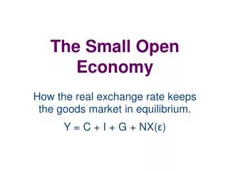
The Small Open Economy. How the real exchange rate keeps the goods market in equilibrium. Y = C + I + G + NX( ε ). Model Background.

E N D
The Small Open Economy How the real exchange rate keeps the goods market in equilibrium. Y = C + I + G + NX(ε)
Model Background • This model is open in the sense that there are exports (X) and imports (M) in the model. Note that net exports (NX) equals (X-M). The model still includes government tax and expenditure. The real exchange rate (not the interest rate) is the equilibrating force in this model. • In other words if the model is out of equilibrium it is the changing real exchange rate that returns the model to equilibrium. • The left hand side of the goods market represents supply. • The right hand side represents demand. Y > C + I + G + NX(ε) => exchange rate decreases => NX increases until Y = C + I + G + NX(ε). Y < C + I + G + NX(ε) => exchange rate increases => NX decreases until Y = C + I + G + NX(ε). Y = C + I + G + NX(ε)
Building the Goods Market Model: supply side Y • This is a long run model so output Y is determined by factor inputs (i.e. K and L) only. • We begin with a production function. • For simplicity we assume K is fixed and allow L to vary. • We get a functional form that is increasing at a decreasing rate. This is consistent with the idea of diminishing marginal returns to labor. • The slope of this function is the marginal product of labor. • It tells us the change in output that results when we increase labor by one unit. Change in Y • We might also assume L is fixed and allow K to vary. • If we chose to combine these images we would get a surface with output on the vertical axis and capital and labor on the other axes. • In this case a cross section of the surface would provide us with the two-dimensional production functions above. Change in L L Y Change in Y Change in K K
Building the Goods Market Model: supply side RealWage • Factor demand is the marginal product of that factor. Labor demand, for example, is defined as the MPL. • The real wage W/P is the real price of labor. Where W (nominal wage) and P (price) are determined exogenously. • To determine the optimal amount of L, firms add L until the MPL = W/P. • This is the profit maximization process that ultimately determines output. • The process is exactly the same for capital K. MPK = R/P (rental rate of capital divided by the price level). (W/P)* MPL is LaborDemand L L* RealRentalRate (R/P)* MPK is CapitalDemand K K*
Building the Goods Market Model: demand side • We begin with consumption, investment, government expenditure, and net exports. This gives us the following national income accounting identity. Y = C + I(r*) + G + NX(ε) …We know Y=F(K,L) • Now, given a savings rate “s” we say c=(1-s) is the marginal propensity to consume. This gives us a consumption function C = c(Y-T). • “r” is the real interest rate. Investment and the real interest rate have a negative relationship so I(r) is negatively sloped. As “r” increases “I” decreases. In this case however it is the world interest rate (r*) that dominates the small open economy. Much like a perfect competitor is a price taker the small open economy is an interest rate taker. Domestic investors always have access to the world interest rates and their economy is so small it can not affect the world interest rate. • “T” is the amount of tax collected. • NX = (X-M) is the trade balance and is dependent on the real exchange rate “ε” From this we get… • Y = c(Y-T) + I(r*) + G + NX(ε) …rearranging we get,Y - c(Y-T) - G = I(r*) + NX(ε) …or,Sn = I(r*) + NX(ε) …orSn - I(r*) = NX(ε) …so national savings - investment = net exports we call (S-I) net capital outflow because when savings is positive it is lent abroad.
Goods Market Equilibrium: The Loanable Funds Market • We said the small open economy model long run equilibrium occurs at the point where Y = c(Y-T) + I(r*) + G + NX(ε) and that if the system is out of equilibrium then “ε” must change to equilibrate the system. • Recall that S - I(r*) = NX(ε) is just a rearrangement of the goods market into net capital flow and trade balance components. This rearrangement is called the loanable funds market. • If the loanable funds market is out of equilibrium then the exchange rate adjusts to equilibrate it which in turn ensures that the goods market is in equilibrium. ε S-I(r*) ε ε ε* NX(ε) S-I(r*),NX(ε)
The Markets in Transition • Things that might shift S-I include changes in Y, T, G, or the mpc. • Things that might shift NX include changes in domestic and foreign trade policy policies such as tariffs or quotas. • There are various effects which can enter the model and change either S-I or NX leading to a change in the real exchange rate. ε S-I(r*) S-I(r*) ε* NX(ε) ε* ε* NX(ε) S-I(r*),NX(ε) All these changes require a different real exchange rate to equilibrate the market.
Conclusion • The small open economy model is a simple static model that allows us to see how the real exchange rate adjusts to keep equilibrium in the loanable funds market which implies equilibrium in the goods market. We also see how various exogenous shocks can affect either (S-I) or NX and therefore lead to a different real exchange rate that equilibrates the goods market.