Download
1 / 23
230 likes | 318 Views
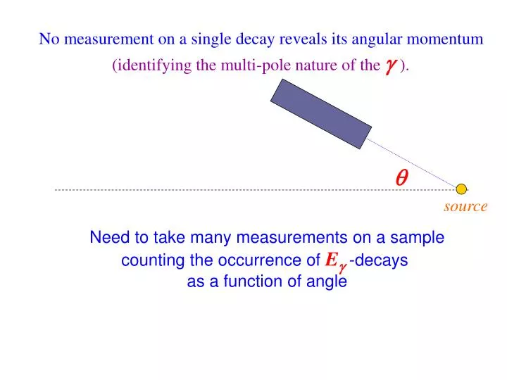
No measurement on a single decay reveals its angular momentum (identifying the multi-pole nature of the g ). . source. Need to take many measurements on a sample counting the occurrence of E g -decays as a function of angle.

E N D
No measurement on a single decay reveals its angular momentum (identifying the multi-pole nature of the g ). source Need to take many measurements on a sample counting the occurrence of Eg -decays as a function of angle
We know, for fixed mjthe radiation is given by the Poynting vector where Same for E and M multipoles
60Co’s -decay to60Niis accompanied by two rapid gamma emissions in succession (lifetimes of ~10-12 sec, make them seem simultaneous) Obviously cascading to its groundstate 60Co ½ = 5.26 years 1g7/2 1g9/2 2p1/2 1f 5/2 2p3/2 1f 7/28 1d3/24 2s1/22 1d5/2628 1p1/22 1p3/24 1s1/22 b- I = ? 2506 keV 4 I = 2+ 1333 keV I = 0+ GROUND 60Ni
60Co’s -decay to60Niis accompanied by two rapid gamma emissions in succession (lifetimes of ~10-12 sec, make them seem simultaneous) 60Co Assuming (trying) different values for I1 would lead you to expect ½ = 5.26 years b- I = ? 2506 keV I1 = 0 I = 2+ 1333 keV I1 = 3 I = 0+ GROUND I1 = 4 60Ni
mj1 = -j1, -j1+1, …, j1-1, j1 Jintial mj2 = -j2, -j2+1, …, j2-1, j2 Jfinal unless special steps taken to orient nuclei the various mjstates are equally populated and mjSjmj = constant
Jintial = 1 mj1 = -1, 0, +1 Jfinal = 0 mj2 = 0 minitial mfinal 0 0 1 0 With the three mj1 states equally populated: Isotropic! independent of .
B-field mi=-1 Ji = 1 mi=-1, 0, +1 mi=0 mi=+1 E+E E E-E Jf = 0 Jf = 0 mf=0 mf=0 E = mB but to compare atomic to nuclear splitting look at one Bohr magneton and the nuclear magneton:
However applying a strong magnetic field to a nuclear system at low temperature can exploit the Boltzmann distribution At kT<<mB the nuclear spins are aligned with the external B-field minitial= +1
At T << B nuclear spins tend to be aligned with the external B Yielding, for example for mi=+1 /2 3/2 2
Description of Nuclear Polarization Polarization
Low temperature Nuclear Orientation At high temperatures ( 1 K !) occupation of the nuclear energy levels are equal. At lower temperatures (100 mK) the lower energy levels are preferentially occupied. For this a 3He:4He dilution refrigerator is widely used.
Measurement of temperature Resistance thermometry3He Melting curve thermometryNuclear orientation thermometry
Nuclear orientationis detected by the temperature-dependent change in the pattern of emitted radiation from appropriate nuclei. most easily measured for the radiation that exits the cryostat walls of the cooling chamber (for low energy and radiation the detectors need to be inside the cryostat). For 60Co, even at 1 K radiation, the pattern of radiation is uniform in all directions.
At lower temperatures the radiation pattern becomes distorted This is most easily detected by a g-detector aligned with the sample axis though frequently an azimuthal detector is also used. An external magnetic field may be needed to sweep out magnetic domains, ensuring all of the target nuclei are correctly aligned.
Ultra Low Temperature Thermometry The equilibrium concentration of 3He/4He is temperature and pressure dependent. The vapor pressure of 3He is higher than 4He Manipulating the 3He/4He concentration (by pumping) can control the temperature. Similar to evaporation techniques in your refrigerator.
The production of low temperatures Evaporation refrigeration using liquid 3He (T~0.3 to 0.5 Kelvin) Dilution refrigeration continuous refrigeration to low temperatures but low cooling power 3He 3He 4He 4He 3He + 4He mixture at T>0.8 K Phase Separation Driven by osmotic pressure differences when temperature is low enough ~0.8 K Dilution and Cooling Driving temperatures lower T0.01 K
Pumping chamber 3He draws 3He out of solution Still return line 3He/4Ne mixture “Sink” Mixing chamber
Angular Correlation Technique Ef -counter Ei-counter source Ji g1 Useful when there is a cascade of successive radiations J g2 Jf After the 1st transition the orientation of atoms is no longer random i.e., not all mj-values for the 2nd transition are equally probable!
Ji As a simple example, consider the special case where Ji= Jf = 0 with an intermediate state of J. g1 J g2 For the initial transition to the intermediate nuclear state mj = J, J-1, …-(J-1), -J are equally likely. Jf Suppose 1 carries off angular momentum 1. It must leave the intermediate nuclear state withmj=-1. ?? Since mf can only = 0, it follows 2 = mj = -1 Nature’s randomly selected 1st step, fixes the nature of the 2nd step.
For example suppose J = 1 mj = -1, 0, +1 Ji g1 J g2 The 1st transition emits 1 leaving the nucleus in one state of mj. Jf Positioning a detector effectively fixes the z-axis, by selecting a direction! When the Ei-counter registers a hit it is selecting p1as the z-axis. ^ Ef -counter Any it detects can’t be from a ~sin2 distribution, only the ~ 1 + cos2. Ei-counter source The Ei-counter preferentially selects out the m=1 decays!
With 1 = 0, the Yjm=Yj0 transition is not even detected. The remaining (equally likely) cases m = 1 have been selected out. The distribution resulting from these two contributions of coincident radiation So if Ji=0, J=1, Jf=0 (the dipole transition Krane uses as an example) or if J=2