Download
1 / 34
340 likes | 476 Views
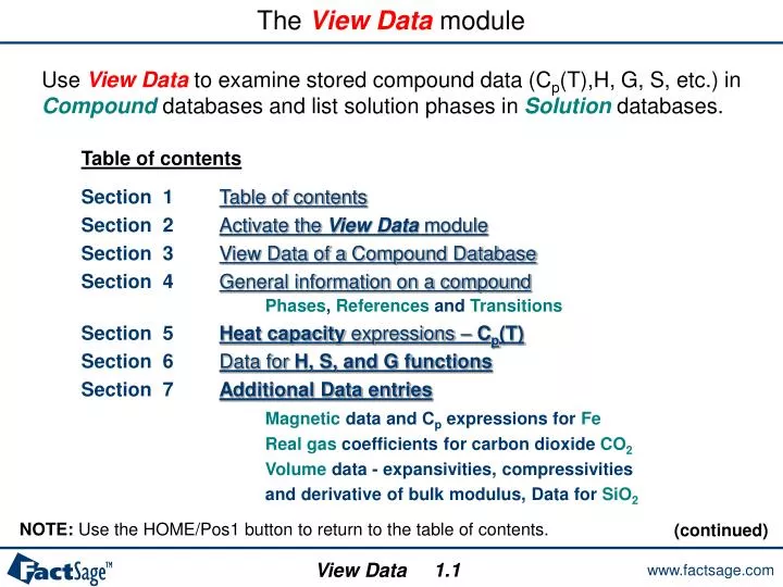
The View Data module. Use View Data to examine stored compound data (C p (T),H, G, S, etc.) in Compound databases and list solution phases in Solution databases. Table of contents. Section 1 Table of contents Section 2 Activate the View Data module

E N D
The View Data module Use View Data to examine stored compound data (Cp(T),H, G, S, etc.) in Compound databases and list solution phases in Solution databases. Table of contents Section 1Table of contents Section 2Activate the View Data module Section 3View Data of a Compound Database Section 4 General information on a compoundPhases,References andTransitions Section 5Heat capacity expressions – Cp(T) Section 6Data for H, S, and G functions Section 7Additional Data entries Magneticdata and Cp expressions forFe Real gascoefficients for carbon dioxideCO2 Volumedata - expansivities, compressivities and derivative ofbulk modulus, Data forSiO2 NOTE: Use the HOME/Pos1 button to return to the table of contents. (continued) View Data 1.1
The View Data module Table of contents (continued) Section 8Executing Calculations: The Menu Bar Tabular output forFe Plotted Cp data forFe Section 9View Data of a Solution Database The solution phase list window Section 10Database Management with View Data Summary Adding a database Removing a database Data search in many databases NOTE: Use the HOME/Pos1 button to return to the table of contents. View Data 1.2
The View Data module Click on View Data in the main FactSage window. View Data 2.0
View Data of a Compound Database In this example, we will scan the FACT slide show compound database for all species of Ca, Al and/or O. 1. Enter the species you wish to view in the database. 3. Select the type of database. 2. Select the units of pressure and energy. 4. Select the database in the drop-down list. Click on «Exit» to close View Data. Click on «Information …» to open FactSage Browser (when available). For database management, see section 10. 5. Click on «OK» to scan the database. View Data 3.1
The List of Compounds Elements specified Units selected Name of the database Menu Bar (more details on the next slide) Number of species in the database Double-click or press «Enter» to view the compound data. List of chemical species frame Location of the database Status of the database Total number of species in the database View Data 3.2
Menu Bar – List of Compounds Menus available with the List of Chemical Species window: Initiate a new search in View Data. Open the «Save As …» dialog box (you can save your data in a text file [*.txt]). Open the «Print…», «Print Setup…» or «Print Font…» dialog boxes (Windows features). Exit the View Data program. Open the «Find…» dialog box. Click to select your units. • Click to list all species containing : • Ca, Al and/or O; • Ca; • Al; • O. Open this slide show. View Data 3.3
The Chemical Species Window: Phases Tab This frame appears after you selected a particular compound in the List of chemical species frame or if you have enter a particular compound in the View Data New Search window. You can display additional data by clicking on the different tabs. Chemical species specified Menu Bar (more details on the next slide) Number of phases in the database for the specified chemical species Species name, formula weight and composition Chemical species frame There are 2 temperature ranges for Al (liquid-1) – each has its own CP expression. • Data retrieved from the database include at least the : • Phases; • Cp(T) polynomial expressions and the derived values of H(T), G(T) and S(T); • Bibliographic references and the standard state transition at 1 atm or bar. References Density View Data 4.1
Menu Bar: Menus available with the Chemical Species window In addition to the menus available in the List of Chemical Species Frame, you can access the Databases, Table and Graph menus. Databases menu lists all the availabledatabases. Data for the current chemical species (here, Al) is retrieved from the checked database (FACT) but data on this chemical species (Al) is also found in other databases. To view the data in another database, click on the database name. The Table and Graph menus enable you to calculate thermodynamic properties and display the values in a tabular or graphical output. See section 8 for an example. View Data 4.2
References and Transitions Tabs Refs. Tab: Complete references Trans. Tab: Standard state transition at 1 atm (or bar, in accordance with your choice of pressure units). View Data 4.3
The basic compound data: H298, S298 and Cp coefficients The following slide shows the basic data that are stored for any compound in a database. These are: • the enthalpy of formation DH298, • the entropy S298 and • the coefficients of the Cp-polynomial In many cases it is necessary to use more than one set of coefficients of Cp in order to describe the Cp-curve with sufficient accuracy. Furthermore, if a compound undergoes phase changes with increasing temperature, each new phase will have at least one new Cp-polynomial expression. View Data 5.0
Heat capacity expressions – Cp(T) • Cp(T) expressions are stored as polynomials in the Cp range [Tmin, Tmax] : • Outside the Cp range: • When T < Tmin, Cp(T) is extrapolated; • When T > Tmax, Cp(T) at Tmax is used. The heat capacity expression of solid aluminum between 298K and 1200K is: Cp(T) = (45.924818 + 1.56972870 × 10⁻⁵T2– 2850.4189 T-1 – 0.77191758 T0.5 - 5945470.3 T-3) [J/mol·K] Note that the 2nd Cp expression for the liquid is constant at temperatures above 1200 K. View Data 5.1
Different derivedthermodynamicfunctions: H(T), S(T) and G(T) The basic data DH298, S298 and Cp(T) can be used to derive the temperature dependence of the enthalpy, H(T), the entropy, S(T) and, most important, the Gibbs energy, G(T). Absolute S(T) can be calculated from the 3rd law: Absolute H(T) is given by : Absolute S(T) and H(T) are combined in the Gibbs-Helmholtz equation: View Data 6.0
Enthalpy H(T), Entropy S(T)and Gibbs Energy G(T)Expressions H(T), G(T) and S(T) are absolute values - not the delta values. For tabular values of Delta H, Delta G and Delta S, use the Reaction module. The enthalpy expression of solid aluminum between 298K and 1200K is: H(T) = (5025.23805 + 45.9248180 T + 5.232429015 × 10⁻⁶T3– 2850.41894 ln(T) – 0.514611719 T1.5 + 2972735.17 T-2) [J/mol] View Data 6.1
Additional basic data of a compound With the compound database it is also possible to store : • data for the magnetic Gibbs energy of a solid compound; • basic data to enable the calculation of virial coefficients of gaseous compounds; • data to treat the pressure dependence of the Gibbs energy of condensed compounds according to the Birch-Murnaghan approach. View Data 7.0
Magnetic data and Cp expressions for Fe Where p is the P Factor and b is the Structure Factor. View Data 7.1
Real gas coefficients for carbon dioxide CO2 Bisestimated (for pure gases and mixtures) by the Tsonopoulosmethod*from Pc, Tc and omega (the acentric factor) for the pure gases. Gases are treated as non-polar. For idealgases, the value of Biszero. * «An Empirical Correlation of Second Virial Coefficients» by C. Tsonopoulos, AIChE Journal, vol. 20, No 2, pp. 263-271, 1974. The truncated virial equation of state is employed to treat real gases: View Data 7.2
Pressure dependence of SiO2 9 phases including 8 solid phases with volume data. View Data 7.3
Volumedata -expansivities,compressibilitiesand bulkmodulus Thermal expansion expression (expansivities) : Compressibility expression (compressibilities) : Derivative of the bulk modulus expression : View Data 7.4
Generation of a tabular output In this example, we will calculate the thermodynamic properties of Fe. 1. Click on the Table menu, and then select the type of phase(s). 2. Click again on the Table menu, select «TK limits (default values) …» and enter the limits of temperature. • Click again on the Table menu and select the command «Table (your selection of phases) …» to generate the table. View Data 8.1
Tabular output for Fe Phase transitions S1S2S1LG as T increases are displayed. The allotropic transformation S1 S2 (alpha gamma) at1184.81 K with an associatedenthalpy of transformation of (34587.3 - 33574.4) = 1012.9 J AtthistemperatureG(S1) = G(S2) (two phases in equilibrium). The allotropic transition reverses at1667.47 Kwhere S2 S1 (gamma delta). The enthalpy of fusion is 13806.9 J at1810.95 K. The enthalpy of vaporization to formmonatomic Fe(g) at 1 atmis (482944.2 – 133371.2) = 349573.0 J at3135.00 K. View Data 8.2
Generation of a graphical output In this example, we will plot the Cp data of Fe. 1. Click on the Graph menu, and then select the type of phase(s). 2. Click again on the Table menu, select «TK limits (default values) …» and enter the limits of temperature. 3. Click again on the Table menu and select the command «Table (your selection of phases) …» to generate the graph. View Data 8.3
Plotted Cp data for Fe View Data uses the Figure Module to generate the graphical output. Curietemperature = 1043 K View Data 8.4
View Data of a Solution Database In this example, we will scan the FACT slide showsolution database for all solutions containing Ca, Al and/or O. 1. Enter the elements. 3. Select the type of database. 2. Select the units of pressure and energy. 4. Select the database in the drop-down list. For database management, see section 10. 5. Click on «OK» to scan the database. View Data 9.1
The solution datasets window Elements specified Name of the database Menu Bar (more details on the next slide) Number of solutions in the database List of solutions frame Location of the database Number of multicomponent solutions in the database Status of the database View Data 9.2
Menu Bar – Solution Datasets Window Menus available with the solution datasets window: Initiate a new search in View Data. Open the «Save As …» dialog box (you can save your data in a text file [*.txt]). Open the «Print…», «Print Setup…» or «Print Font…» dialog boxes (Windows features). Exit the View Data program. Open the «Find…» dialog box (Windows features). Click to select your units. • Click to view a list of all solutions containing : • Ca, Al and/or O; • Ca; • Al; • O. You can use the Summary Menu to narrow your search (for example, all solutions containing Ca). Note: You can not access the Databases, Table and Graph menus in the Solution Datasetswindow. Open this slide show. View Data 3.3
Database Management using View Data The following slides show how the View Data module is used to link additional Compound and Solution databases to FactSage. Once other databases are linked with FactSage it is possible to use them in combined searches for compounds or solutions datasets. The result of such a combined search is shown. View Data 10.0
View Data New Search window Databases Frame Click on «Summary…» to open the Summary of Databases window. Click on «Add…» to open the List of Databases window. Here there are 19 compound databases on the search list. Your PC will not have all of them. Scroll down to view a list of their nicknames. Click on «Remove…» to remove a database from the list. (The database is not erased from your computer, it is only removed from the list) View Data 10.1
Summary of Databases Window The summary of databases gives the current status of all databases available on your computer. View Data 10.2
List of Databases Window Select the Database Type to add. Click on «Summary…» to open the Summary of Databases window. Filename including the path. Description (one line) of the selected database. Nickname (4 characters) of the selected database. Click on «Scan …» to scan through the /FACTDATA directory and identify databases that are not already on the list. Click on «Browse…» to open the All databases dialog box. View Data 10.3
Add database to the list 1. Select the Database Type to add. • Enter the database to add by: • Typing the complete filename (including the path); or, • Click on «Browse…» to open the All databases dialog box; or, • Click on «Scan …» to scan through the /FACTDATA directory and identify databases that are not already on the list. View Data 10.4
Add database to the list using the «Browse…» button 1. Select the Database Type to add. 3. Select a database and click on «Open». • Click on «Browse…» to open the All databasesdialog box. Click on «OK» to add to the list. You mayedit and change the info. You canadd more databases to the list (return to step 1) or click on «Quit» to finish addingdatabases. View Data 10.5
Add database to the list using the «Scan…» button 1. Select the Database Type to add. • Click on «Scan…» to scan through the /FACTDATA directory and identifydatabasesthat are not already on the list. Note: This is a read-onlydatabase. 3. Click on «OK» to add to the list. If the selected database is coupled with another one, View Data will prompt you. In the case of coupleddatabases, itisusuallywise to answer «Yes». You canadd more databases to the list (return to step 1) or click on «Quit» to finish. View Data 10.6
Removing a database from the list To remove a database: 1. Select the type of database in the View Data window. 2. Select the database you wish to remove from the drop-down menu. 3. Click on «Remove…». • 4. View Data will prompt you: • If the selected database is not coupled with another one. • If the selected database is coupled with another one. Yeswill remove the BINS Compound database. Yeswill remove both (compound and solution) database. Nowill remove your selection of the type of database made in step 1. View Data 10.7
Search in more than one database 1. To search more than one database, select the option «All Databases» in the scroll down list. Note: You can use the «Add…» and «Remove…» features to expand or narrow the number of databases included in your search. View Data 10.8