rel. to max length age 10

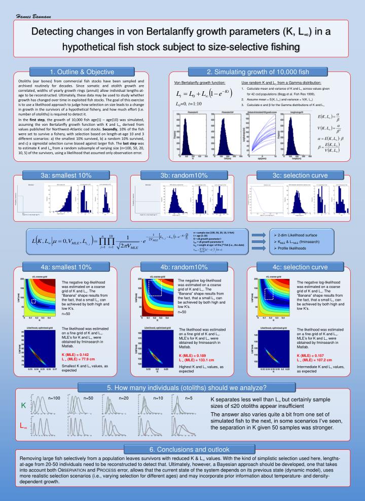
1. Hannes Baumann Detecting changes in von Bertalanffy growth parameters (K, L∞) in a hypothetical fish stock subject to size-selective fishing 1. Outline & Objective 2. Simulating growth of 10,000 fish Otoliths (ear bones) from commercial fish stocks have been sampled and archived routinely for decades. Since somatic and otolith growth are correlated, widths of yearly growth rings (annuli) allow individual lengths-at-age to be reconstructed. Ultimately, these data may be used to study whether growth has changed over time in exploited fish stocks. The goal of this exercise is to use a likelihood approach to judge how selection on size leads to a change in growth in the survivors of a hypothetical fishery, and how much effort (i.e. number of otoliths) is required to detect it. In the first step, the growth of 10,000 fish age(1) – age(10) was simulated, assuming the von Bertalanffy growth function with K and L∞derived from values published for Northwest-Atlantic cod stocks. Secondly, 10% of the fish were set to survive a fishery, with selection based on length-at-age 10 and 3 different scenarios: a) the smallest 10% survived, b) a random 10% survived, and c) a sigmoidal selection curve biased against larger fish. The last step was to estimate K and L∞ from a random subsample of varying size (n=100, 50, 20, 10, 5) of the survivors, using a likelihood that assumed only observation error. Von Bertalanffy growth function: Use random K and L∞ from a Gamma distribution: Calculate mean and variance of K and L∞ across values given for 42 cod populations (Begg et al. Fish Res 1999), Assume mean = E(K, L∞) and variance = V(K, L∞) Calculate α and β for the Gamma distributions of K and L∞ L0=0, t=1:10 3a: smallest 10% 3b: random10% 3c: selection curve rel. to max length age 10 Selection Selection Probability of selection Probability of selection • 2-dim Likelihood surface • KMLE & L∞MLE (fminsearch) • Profile likelihoods n = sample size (100, 50, 20, 10, 5 fish) t = age (1-10) K = vB growth parameter I Linf = vB growth parameter II Lti,j = Length at age i of the jth fish (i.e., the data) 0.1 length rel. to max length age 10 length rel. to max length age 10 4a: smallest 10% 4b: random10% 4c: selection curve The negative log-likelihood was estimated on a coarse grid of K and L∞. The “Banana” shape results from the fact, that a small L∞ can be achieved by both high and low K’s. n=50 The negative log-likelihood was estimated on a coarse grid of K and L∞. The “Banana” shape results from the fact, that a small L∞ can be achieved by both high and low K’s. The negative log-likelihood was estimated on a coarse grid of K and L∞. The “Banana” shape results from the fact, that a small L∞ can be achieved by both high and low K’s. n=50 The likelihood was estimated on a fine grid of K and L∞. MLE’s for K and L∞ were obtained by fminsearch in Matlab. K (MLE) = 0.142 L ∞ (MLE) = 77.9 cm The likelihood was estimated on a fine grid of K and L∞. MLE’s for K and L∞ were obtained by fminsearch in Matlab. K (MLE) = 0.189 L ∞ (MLE) = 133.1 cm The likelihood was estimated on a fine grid of K and L∞. MLE’s for K and L∞ were obtained by fminsearch in Matlab. K (MLE) = 0.157 L ∞ (MLE) = 107.2 cm Smallest K and L∞ values, as expected Highest K and L∞ values, as expected Intermediate K and L∞ values, as expected 5. How many individuals (otoliths) should we analyze? n=100 n=50 n=20 n=10 n=5 K separates less well than L∞ but certainly sample sizes of ≤20 otoliths appear insufficient The answer also varies quite a bit from one set of simulated fish to the next, in some scenarios I’ve seen, the separation in K given 50 samples was stronger. K L∞ 6. Conclusions and outlook Removing large fish selectively from a population leaves survivors with reduced K & L∞ values. With the kind of simplistic selection used here, lengths-at-age from 20-50 individuals need to be reconstructed to detect that. Ultimately, however, a Bayesian approach should be developed, one that takes into account both Observation and Process error, allows that the current state of the system depends on its previous state (dynamic model), uses more realistic selection scenarios (i.e., varying selection for different ages) and may incorporate prior information about temperature- and density-dependent growth.