Download
1 / 19
210 likes | 257 Views
Numerical Differentiation. Numerical Differentiation. First order derivatives High order derivatives Examples. Motivation. How do you evaluate the derivative of a tabulated function. How do we determine the velocity and acceleration from tabulated measurements. Recall.

E N D
Numerical Differentiation First order derivatives High order derivatives Examples
Motivation • How do you evaluate the derivative of a tabulated function. • How do we determine the velocity and acceleration from tabulated measurements.
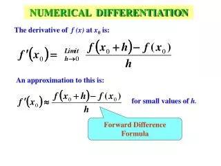
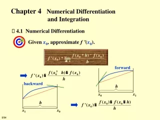
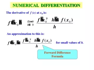
For small values of h, the difference quotient [f (x0 + h) − f (x0)]/h can be used to approximate f’(x0) with an error bounded by M|h|/2, where M is a bound on |f’’(x)| for x between x0 and x0 +h.
Example • Use forward, backward and centered difference approximations to estimate the first derivate of: f(x) = –0.1x4 – 0.15x3 – 0.5x2 – 0.25x + 1.2 at x = 0.5 using step size h = 0.5 and h = 0.25 • Note that the derivate can be obtained directly: f’(x) = –0.4x3 – 0.45x2 – 1.0x – 0.25 The true value of f’(0.5) = -0.9125 • In this example, the function and its derivate are known. However, in general, only tabulated data might be given.
Solution with Step Size = 0.5 • f(0.5) = 0.925, f(0) = 1.2, f(1.0) = 0.2 • Forward Divided Difference: f’(0.5) (0.2 – 0.925)/0.5 = -1.45 |t| = |(-0.9125+1.45)/-0.9125| = 58.9% • Backward Divided Difference: f’(0.5) (0.925 – 1.2)/0.5 = -0.55 |t| = |(-0.9125+0.55)/-0.9125| = 39.7% • Centered Divided Difference: f’(0.5) (0.2 – 1.2)/1.0 = -1.0 |t| = |(-0.9125+1.0)/-0.9125| = 9.6%
Solution with Step Size = 0.25 • f(0.5)=0.925, f(0.25)=1.1035, f(0.75)=0.6363 • Forward Divided Difference: f’(0.5) (0.6363 – 0.925)/0.25 = -1.155 |t| = |(-0.9125+1.155)/-0.9125| = 26.5% • Backward Divided Difference: f’(0.5) (0.925 – 1.1035)/0.25 = -0.714 |t| = |(-0.9125+0.714)/-0.9125| = 21.7% • Centered Divided Difference: f’(0.5) (0.6363 – 1.1035)/0.5 = -0.934 |t| = |(-0.9125+0.934)/-0.9125| = 2.4%
Discussion • For both the Forward and Backward difference, the error is O(h) • Halving the step size h approximately halves the error of the Forward and Backward differences • The Centered difference approximation is more accurate than the Forward and Backward differences because the error is O(h2) • Halving the step size h approximately quarters the error of the Centered difference.
Example 2 Use the forward-difference formula to approximate the derivative of f (x) = ln x at x0 = 1.8 using h = 0.1, h = 0.05, and h = 0.01, and determine bounds for the approximation errors.
Solution The forward-difference formula f (1.8 + h) − f (1.8) h with h = 0.1 gives (ln 1.9 − ln 1.8)/0.1 = (0.64185389 − 0.58778667)/0.1 = 0.5406722. Because f’’(x) = −1/x2and 1.8 < ξ < 1.9, a bound for this approximation error is |hf’’(ξ )|/2 =|h|/2ξ2<0.1/2(1.8)2= 0.0154321.