Download
1 / 36
370 likes | 604 Views
Bottom-up Parsing. Parsing Techniques. Top-down parsers (LL(1), recursive descent) Start at the root of the parse tree and grow toward leaves Pick a production & try to match the input Bad “pick” may need to backtrack

E N D
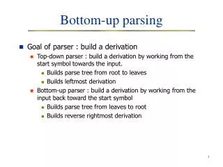
Parsing Techniques Top-down parsers (LL(1), recursive descent) Start at the root of the parse tree and grow toward leaves Pick a production & try to match the input Bad “pick” may need to backtrack Some grammars are backtrack-free (predictive parsing) Bottom-up parsers (LR(1), operator precedence) Start at the leaves and grow toward root As input is consumed, encode possibilities in an internal state Start in a state valid for legal first tokens Bottom-up parsers handle a large class of grammars
Bottom-up Parsing(definitions) The point of parsing is to construct a derivation A derivation consists of a series of rewrite steps S 0 1 2 … n–1 nsentence • Each i is a sentential form • If contains only terminal symbols, is a sentence in L(G) • If contains ≥ 1 non-terminals, is a sentential form • To get i from j–1, expand some NT A i–1by using A • Replace the occurrence of A i–1with to get i • In a leftmost derivation, it would be the first NT Ai–1 A left-sentential formoccurs in a leftmost derivation A right-sentential form occurs in a rightmost derivation
Bottom-up Parsing • Bottom-up paring and reverse right most derivation • A derivation consists of a series of rewrite steps • A bottom-up parser builds a derivation by working from the input sentence back toward the start symbol S S 0 1 2 … n–1 nsentence In terms of the parse tree, this is working from leaves to root • Nodes with no parent in a partial tree form its upper fringe • Since each replacement of with A shrinks the upper fringe, we call it a reduction. Bottom-up
Finding Reductions (Handles) The parser must find a substring of the tree’s frontier that matches some production A that occurs as one step In the rightmost derivation Informally, we call this substring a handle Formally, A handle of a right-sentential form is a pair <A,k> where A P and k is the position in of ’s rightmost symbol. If <A,k> is a handle, then replace at k with A Handle Pruning The process of discovering a handle and reducing it to the appropriate left-hand side is called handle pruning Because is a right-sentential form, the substring to the right of a handle contains only terminal symbols
Example (a very busy slide) The expression grammar Handles for rightmost derivation of x–2*y
How do errors show up? • failure to find a handle • hitting EOF & needing to • shift (final else clause) • Either generates an error Handle-pruning, Bottom-up Parsers One implementation technique is the shift-reduce parser push INVALID token next_token( ) repeat until (top of stack = Goal and token = EOF) if the top of the stack is a handle A then /* reduce to A*/ pop || symbols off the stack push A onto the stack else if (token EOF) then /* shift */ push token token next_token( )
Back to x-2*y 5 shifts + 9 reduces + 1 accept 1. Shift until the top of the stack is the right end of a handle 2. Find the left end of the handle & reduce
Back to x-2*y 5 shifts + 9 reduces + 1 accept 1. Shift until the top of the stack is the right end of a handle 2. Find the left end of the handle & reduce
Back to x-2*y 5 shifts + 9 reduces + 1 accept 1. Shift until the top of the stack is the right end of a handle 2. Find the left end of the handle & reduce
Back to x-2*y 5 shifts + 9 reduces + 1 accept 1. Shift until the top of the stack is the right end of a handle 2. Find the left end of the handle & reduce
Back to x-2*y 5 shifts + 9 reduces + 1 accept 1. Shift until the top of the stack is the right end of a handle 2. Find the left end of the handle & reduce
Back to x–2*y 5 shifts + 9 reduces + 1 accept 1. Shift until the top of the stack is the right end of a handle 2. Find the left end of the handle & reduce
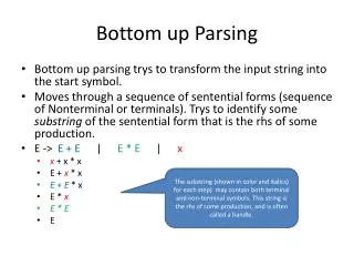
Goal Expr Expr Term Term Term Fact. Fact. Fact. Example – * <id,y> <id,x> <num,2>
Shift-reduce Parsing Shift reduce parsers are easily built and easily understood A shift-reduce parser has just four actions • Shift — next word is shifted onto the stack • Reduce— right end of handle is at top of stack Locate left end of handle within the stack Pop handle off stack & push appropriate lhs • Accept—stop parsing & report success • Error— call an error reporting/recovery routine Critical Question: How can we know when we have found a handle without generating lots of different derivations? • Answer: we use look ahead in the grammar along with tables produced as the result of analyzing the grammar. • LR(1) parsers build a DFA that runs over the stack & find them • Handle finding is key • handle is on stack • finite set of handles • use a DFA !
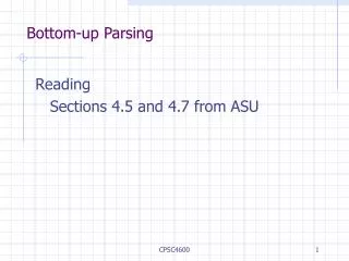
LR(1) Parsers A table-driven LR(1) parser looks like Tables canbe built by hand It is a perfect task to automate Scanner Table-driven Parser ACTION & GOTO Tables Parser Generator source code IR grammar
LR(1) Skeleton Parser stack.push(INVALID); stack.push(s0); not_found = true; token = scanner.next_token(); do while (not_found) { s = stack.top(); if ( ACTION[s,token] == “reduceA” ) then { stack.popnum(2*||); // pop 2*|| symbols s = stack.top(); stack.push(A); stack.push(GOTO[s,A]); } else if ( ACTION[s,token] == “shift si” ) then { stack.push(token); stack.push(si); token scanner.next_token(); } else if ( ACTION[s,token] == “accept” & token == EOF ) then not_found = false; else report a syntax error and recover; } report success; • The skeleton parser • uses ACTION & GOTO tables • does |words| shifts • does |derivation| • reductions • does 1 accept • detects errors by failure of 3 other cases
LR(1) Parsers How does this LR(1) stuff work? Unambiguous grammar unique rightmost derivation Keep upper fringe on a stack All active handles include top of stack (TOS) Shift inputs until TOS is right end of a handle Language of handles is regular (finite) Build a handle-recognizing DFA ACTION & GOTO tables encode the DFA To match subterm, invoke subterm DFA & leave old DFA’s state on stack Final state in DFA a reduce action New state is GOTO[state at TOS (after pop), lhs] For SN, this takes the DFA to s1 Reduce action baa S1 S3 SN S0 baa Reduce action S2 Control DFA for SN
Building LR(1) Parsers How do we generate the ACTION and GOTO tables? Use the grammar to build a model of the DFA Use the model to build ACTION & GOTO tables If construction succeeds, the grammar is LR(1) The Big Picture Model the state of the parser Use two functions goto( s, X ) and closure( s ) goto() is analogous to move() in the subset construction closure() adds information to round out a state Build up the states and transition functions of the DFA Use this information to fill in the ACTION and GOTO tables Terminal or non-terminal
LR(k)items An LR(k) item is a pair [P, ], where P is a production A with a • at some position in the rhs is a lookahead string of length ≤ k(words or EOF) The • in an item indicates the position of the top of the stack [A•,a] means that the input seen so far is consistent with the use of A immediately after the symbol on top of the stack [A •,a] means that the input sees so far is consistent with the use of A at this point in the parse, and that the parser has already recognized . [A •,a] means that the parser has seen , and that a lookahead symbol of a is consistent with reducing to A. The table construction algorithm uses items to represent valid configurations of an LR(1) parser
Computing Gotos Goto(s,x) computes the state that the parser would reach if it recognized an x while in state s • Goto( { [AX,a] }, X) produces [AX,a] (obviously) • It also includes closure( [AX,a] ) to fill out the state The algorithm • Not a fixed point method! • Straightforward computation • Uses closure( ) • Goto() advances the parse Goto( s, X ) new Ø items [A•X,a] s new new [AX•,a] return closure(new)
Computing Closures Closure(s) adds all the items implied by items already in s • Any item [AB,a] implies [B,x] for each production with B on the lhs, and each x FIRST(a) • Since B is valid, any way to derive B is valid, too The algorithm Closure( s ) while ( s is still changing ) items [A •B,a] s productionsB P b FIRST(a) // might be if [B • ,b] s then add [B • ,b] to s • Classic fixed-point algorithm • Halts because s ITEMS • Worklist version is faster • Closure “fills out” a state
LR(1) Items The production A, where = B1B1B1 with lookahead a, can give rise to 4 items [A•B1B1B1,a], [AB1•B1B1,a], [AB1B1•B1,a], & [AB1B1B1•,a] The set of LR(1) items for a grammar is finite What’s the point of all these lookahead symbols? Carry them along to choose correct reduction (if a choice occurs) Lookaheads are bookkeeping, unless item has • at right end Has no direct use in [A•,a] In [A•,a], a lookahead of a implies a reduction by A For { [A•,a],[B•,b] }, areduce to A; FIRST() shift Limited right context is enough to pick the actions
LR(1) Table Construction High-level overview • Build the canonical collection of sets of LR(1) Items, I • Begin in an appropriate state, s0 • [S’ •S,EOF], along with any equivalent items • Derive equivalent items as closure( i0 ) • Repeatedly compute, for each sk, and each X, goto(sk,X) • If the set is not already in the collection, add it • Record all the transitions created by goto( ) This eventually reaches a fixed point • Fill in the table from the collection of sets of LR(1) items The canonical collection completely encodes the transition diagram for the handle-finding DFA
Building the Canonical Collection Start from s0= closure( [S’S,EOF] ) Repeatedly construct new states, until all are found The algorithm s0 closure( [S’S,EOF] ) S { s0 } k 1 while ( S is still changing ) sj S and x ( T NT ) sk goto(sj,x) record sj sk on x if sk S then S S sk k k + 1 • Fixed-point computation • Loop adds to S • S 2ITEMS, so S is finite • Worklist version is faster
Example (grammar & sets) Simplified, right recursive expression grammar Goal Expr Expr Term – Expr Expr Term Term Factor * Term Term Factor Factor ident
Example (building the collection) Initialization Step s0 closure( {[Goal •Expr , EOF] } ) { [Goal • Expr , EOF], [Expr • Term – Expr , EOF], [Expr • Term , EOF], [Term • Factor * Term , EOF], [Term • Factor * Term , –], [Term • Factor , EOF], [Term • Factor , –], [Factor • ident , EOF], [Factor • ident , –], [Factor • ident , *] } S {s0 }
Example (building the collection) Iteration 1 s1 goto(s0 , Expr) s2 goto(s0 , Term) s3 goto(s0 , Factor) s4 goto(s0 , ident) Iteration 2 s5 goto(s2 , – ) s6 goto(s3 , * ) Iteration 3 s7 goto(s5 , Expr ) s8 goto(s6 , Term )
Example (Summary) S0 : { [Goal • Expr , EOF], [Expr • Term – Expr , EOF], [Expr • Term , EOF], [Term • Factor * Term , EOF], [Term • Factor * Term , –], [Term • Factor , EOF], [Term • Factor , –], [Factor • ident , EOF], [Factor • ident , –], [Factor • ident, *] } S1 : { [Goal Expr •, EOF] } S2 : { [Expr Term • – Expr , EOF], [Expr Term •, EOF] } S3 : { [Term Factor • * Term , EOF],[Term Factor • * Term , –], [Term Factor •, EOF], [Term Factor •, –] } S4 : { [Factor ident •, EOF],[Factorident •, –], [Factorident •, *] } S5 : { [Expr Term – • Expr , EOF], [Expr • Term – Expr , EOF], [Expr • Term , EOF], [Term • Factor * Term , –], [Term • Factor , –], [Term • Factor * Term , EOF], [Term • Factor , EOF], [Factor • ident , *], [Factor • ident , –], [Factor • ident , EOF] }
Example (Summary) S6 : { [Term Factor * • Term , EOF], [Term Factor * • Term , –], [Term • Factor * Term , EOF], [Term • Factor * Term , –], [Term • Factor , EOF], [Term • Factor , –], [Factor •ident , EOF], [Factor •ident , –], [Factor •ident , *] } S7: { [Expr Term – Expr •, EOF] } S8 : { [Term Factor * Term•, EOF], [Term Factor * Term•, –] }
Filling in the ACTION and GOTO Tables The algorithm Many items generate no table entry • Closure( ) instantiates FIRST(X) directly for [A•X,a ] set sxS item isx if i is [A •ad,b] and goto(sx,a) = sk , aT then ACTION[x,a] “shift k” else if i is [S’S •,EOF] then ACTION[x ,a] “accept” else if i is [A •,a] then ACTION[x,a] “reduce A” n NT if goto(sx ,n) = sk then GOTO[x,n] k x is the state number
Example (Summary) The Goto Relationship (from the construction)
Example (Filling in the tables) The algorithm produces the following table
What can go wrong? What if set s contains [A•a,b] and [B•,a] ? First item generates “shift”, second generates “reduce” Both define ACTION[s,a] — cannot do both actions This is a fundamental ambiguity, called a shift/reduce error Modify the grammar to eliminate it (if-then-else) Shifting will often resolve it correctly What is set s contains [A•, a] and [B•, a] ? Each generates “reduce”, but with a different production Both define ACTION[s,a] — cannot do both reductions This is a fundamental ambiguity, called a reduce/reduce conflict Modify the grammar to eliminate it (PL/I’s overloading of (...)) In either case, the grammar is not LR(1)
LR(k) versus LL(k) (Top-down Recursive Descent ) Finding Reductions LR(k) Each reduction in the parse is detectable with the complete left context, the reducible phrase, itself, and the k terminal symbols to its right LL(k) Parser must select the reduction based on The complete left context The next k terminals Thus, LR(k) examines more context “… in practice, programming languages do not actually seem to fall in the gap between LL(1) languages and deterministic languages” J.J. Horning, “LR Grammars and Analysers”, in Compiler Construction, An Advanced Course, Springer-Verlag, 1976
Summary Top-down recursive descent Advantages Fast Good locality Simplicity Good error detection Fast Deterministic langs. Automatable Left associativity Disadvantages Hand-coded High maintenance Right associativity Large working sets Poor error messages Large table sizes LR(1)