Download

1 / 15

E N D
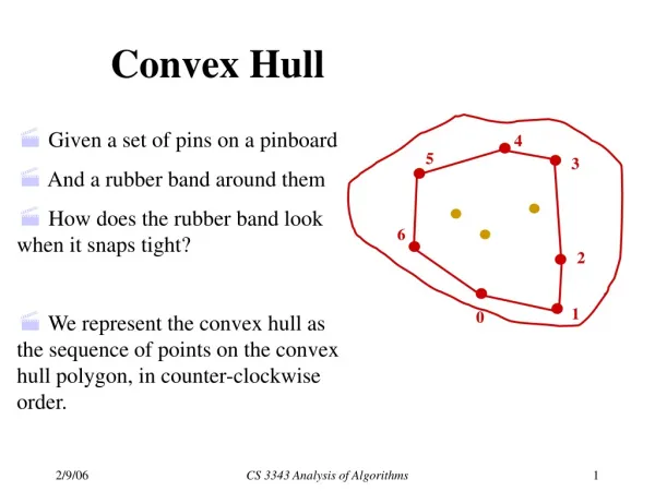
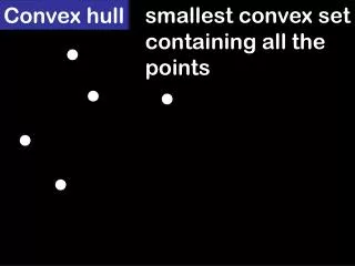
What is the Convex Hull? • Imagine a set of points on a board with a nail hammered into each point. Now stretch a rubber band over all the nails, let go, and the rubber band will form a shape around the outermost nails, encompassing the rest. The shape formed is known as the convex hull. • Formerly, the convex hull of a set of points X in a real vector space V is the smallest convex set containing X. • An object is convex if for every pair of points within the object, every point on the straight line segment that joins them is also within the object. • If a polygon contains angles of 180 degrees or more, it is not convex.
Basic Concepts • If the set of points given contains only one point, that point is its own convex hull. • The convex hull of two unique points is the line segment between the two points. • The convex hull of three nonlinear points is the triangle formed by these three points. If the points are collinear, the convex hull is the line segment connecting the points with the endpoints as extreme points. • An extreme point is a point that lies on the convex hull. In other words, one of the vertices on the polygon that the hull forms. • Four extreme points are obvious when given a set those to the furthest right and left, and those at the top and bottom. • Computational geometry is defined as the study of algorithms to solve problems in computer science in terms of geometry. There are several different algorithms with different efficiencies used to solve the problem of the convex hull.
Jarvis March • Also known as the “gift wrapping” technique. • Start at some extreme point on the hull. • In a counterclockwise fashion, each point within the hull is visited and the point that undergoes the largest right-hand turn from the current extreme point is the next point on the hull. • Finds the points on the hull in the order in which they appear. • Example: http://www.cs.princeton.edu/courses/archive/spr10/cos226/demo/ah/JarvisMarch.html
Implementation • In order to find the biggest right hand turn, the last two points added to the hull, p1 and p2, must be known. • Assuming p1 and p2 are known, the angle these two points form with the remaining possible hull points is calculated. The point that maximizes the angle is the next point in the hull. • To do this, we have two line segments p0p1 and p1p2. We are trying to determine the value of the right hand turn at p1. To do this we find the cross product of (p1 – p0) x (p2 – p0). The point that gives the largest value in this calculation is the next point on the hull. • Continue to make right turns until the original point is reached and the hull is complete.
Efficiency • Proposed by R.A. Jarvis in 1973 • O(nh) complexity, with n being the total number of points in the set, and h being the number of points that lie in the convex hull. • This implies that the time complexity for this algorithm is the number of points in the set multiplied by the number of points in the hull • The worst case for this algorithm is denoted by O(n2), which is not optimal. • Favorable conditions in which to use the Jarvis march include problems with a very low number of total points, or a low number of points on the convex hull in relation to the total number of points.
Graham’s Scan • Sort points by increasing y-coordinate values. In the case of a tie, the leftmost x-coordinate value comes first. This known as the anchor point. • In Graham’s scan, the remaining points in the set are then sorted in increasing order of the angle made by the x-axis, the point P, and the point in the remaining set. • Therefore, the points furthest right with the smallest angles formed will be the first points in the sort, while the points lying furthest to the left will be the last points. • http://www.cs.princeton.edu/courses/archive/fall08/cos226/demo/ah/GrahamScan.html
Graham’s Scan • Once the points are sorted in order in respect to the anchor point from rightmost to leftmost, the anchor point and the point lying furthest to the right (the first point in the sorted data) must both be on the hull. • These two points serve as our initial points on the hull and are pushed onto a stack representing hull points. • From here, for each consecutive point in the sort, it is determined whether a right or left turn is taken from the top two items on the stack to the point. (cross product). • As long as a left hand turn is made, push the point onto the stack. • When a right hand turn is made, pop top point off the stack, reevaluate and continue popping as long as right hand turns are made. Then push the new point onto the stack. • When the initial point is reached again, the points on the stack represent the convex hull.
Pseudocode # Points[1] is the pivot or anchor point Stack.push(Points[1]); Stack.push(Points[2]); FOR I = 3 TO Points.length o = Cross_product(Stack.second, Stack.top, Points[i]; IF o == 0 THEN Stack.pop; Stack.push(Points[i]); ELSE WHILE o <= 0 and Stack.length > 2 Stack.pop; o = Cross_product(Stack.second, Stack.top, Points[i]); ENDWHILE Stack.push(Points[i]); NEXT i
Efficiency • In the Graham Scan, the first phase of sorting points by angle around the anchor point is of time O( n logn) complexity. • Phase 2 of this algorithm has a time complexity of O(n). • The total time complexity for this algorithm is O( n logn) which is much more efficient than a worse case scenario of Jarvis march at O(n2).
Divide and Conquer • In this method, two separate hulls are created, one for the leftmost half of the points, and one for the rightmost half. • To divide in halves, sort by x-coordinates and find the median. If there is an odd number of points, the leftmost half should have the extra point. • Recursively find the convex hull for the left set of points and the right set of points. This gives hull A and hull B. • Stitch together the two hulls to form the hull of the entire set. • http://www.cse.unsw.edu.au/~lambert/java/3d/divideandconquer.html
Implementation • To stitch the hulls together, the upper and lower tangent lines must be found. • To find the lower tangent, start with the rightmost point in hull B and the leftmost point in hull A. While the line segment formed between these two points is not the lower tangent line of the hull, figure which of the two points is not at its lower tangent point. • While A is not the lower tangent point, move around the hull clockwise, that is A=A – 1. • While B is not at the lower tangent point, move around the hull counterclockwise, that is B = B + 1. • When the upper and lower tangent lines are found, march around hull A and hull B deleting the points that are now within the merged convex hull.
Efficiency • The divide and conquer algorithm is also of time complexity O( n logn). • This algorithm is often used for cases in three dimensions. • A technicality of the divide and conquer method lies in how many points are in the set. If the set has less than four points, there is no need to sort the points, but rather for these special cases, determine the hull separately. • A downside to this algorithm is the overhead associated with recursive function calls.
Quickhull • Interactive, redraw as you go algorithm. • Similar to quicksort in efficiency. • Sort in terms of increasing x-coordinate values. • Find four extreme points and form a quadrilateral. • Discard all points that lie within the quadrilateral. • Each edge of the quadrilateral is then examined to see whether any points lie outside the edge of the current hull. • A triangle is drawn from the edge to the point that lies the furthest outside of the edge. Any points within this triangle are eliminated because they do not lie on the hull. • The original edge is removed and new edges are formed with the new point and two closest extreme points. • Edges added to a bucket from which recursion takes place to find any points that lie outside the edge and drawing new triangles until all points are eliminated other than the vertices of the hull. • http://www.cs.princeton.edu/courses/archive/spr10/cos226/demo/ah/QuickHull.html
Efficiency • Proposed by Preparata and Hong in 1977 • Quickhull method exhibits O( n logn) complexity. • For unfavorable inputs, the worst case can be O(n2). • Overall, this algorithm is dependent upon how evenly the points are split at each stage. At times this algorithm can be more useful than Graham’s scan, but if the points are not evenly distributed then it is often not. • Points uniformly distributed in a square can throw out all inner points in only a few iterations. • The quickhull algorithm saves time in that the quicksort of the points (splitting then into an upper and lower hull) splits the problem into two smaller sub-problems that are solved the same way. • It also saves time due to the fact that a significant amount of points that lie within the quadrilateral formed can be eliminated immediately. • The main disadvantage to this algorithm is the overhead associated with recursive function calls.