Download
1 / 21
210 likes | 301 Views
SELFE: Semi-implicit Eularian-Lagrangian finite element model for cross scale ocean circulation. Paper by Yinglong Zhang and Antonio Baptista Presentation by Charles Seaton All figures from paper unless otherwise labeled. Comparison of model types.

E N D
SELFE: Semi-implicit Eularian-Lagrangian finite element model for cross scale ocean circulation Paper by Yinglong Zhang and Antonio Baptista Presentation by Charles Seaton All figures from paper unless otherwise labeled
Comparison of model types • Structured grids, FD: ROMS, POM, NCOM: Good for ocean modeling, require small timesteps, not capable of representing coastline details • Unstructured grids, FE (previous): ADCIRC, QUODDY: Archaic, don’t solve primitive equations • Unstructured grids, FV: UNTRIM-like models: require orthogonality, low order SELFE: Unstructured grids, FE: higher order, does solve primitive equations, can follow coastlines
SELFE: equations continuity Tidal force Baroclinic barotropic Verticalviscosity Horizontalviscosity Atmospheric coriolis Vertical and horizontal diffusion
Turbulence Closure vertical diffusion, vertical and horizontal viscosity dissipation Length scale, 0.3, TKE, mixing length Modelparameters Stability functions Boundary conditions
Vertical Boundary Condition for Momentum Surface Bed Bottom boundary layer velocity Stress in boundary layer Continued next slide
Vertical Boundary Condition for Momentum (continued) Constant stress = 0
Numerical methods • Horizontal grid: unstructured • Vertical grid: hybrid s-z • Time stepping: semi-implicit • Momentum equation and continuity equation solved simultaneously (but decoupled) • Finite Element, advection uses ELM • Transport equation: FE, advection uses ELM or FVUM
s-z vertical grid Can be pure s, can’t be pure z Allows terrain following at shallow depths, avoids baroclinic instability at deeper depths
Grid Prisms w u,v elevation S,T FVUM S,T ELM
Depth averaged momentum Implicit terms Explicit terms Need to eliminate = 0
Momentum Viscosity Viscocity – implicit Pressure gradient – implicit Velocity at nodes = weighted average of velocity at side centers Or use discontinuous velocities Vertical velocity solved by FV
Baroclinic module Transport: ELM or FVUM (element splitting or quadratic interpolation reduces diffusion in ELM) FVUM for Temperature Stability constraint (may force subdivision of timesteps)
Stability From explicit baroclinic terms From explicit horizontal viscosity
Benchmarks • 1D convergence • 3D analytical test • Volume conservation test • Simple plume generation test
1D Convergence • With fixed grid, larger timesteps produce lower errors • Convergence happens only with dx and dt both decreasing • Changing gridsize produces 2nd order convergence in SELFE, but produces divergence in ELCIRC (non-orthogonal grid)
3D quarter annulus • M2 imposed as a function of the angle velocity ELCIRC SELFE
Volume conservation • River discharge through a section of the Columbia
Plume Demonstrates need for hybrid s-z grid
40 100 500 1000