Download

1 / 13
140 likes | 296 Views
Quantifying the Bessel Beam. Josh Nelson. Motivation. Ultimately we want to understand the Bessel beam we send into fiber optics. Thus, we must quantify our Bessel beam using a fitting algorithm There is no already made one so it must coded. Before the code. Slicing Normalizing.

E N D
Quantifying the Bessel Beam Josh Nelson
Motivation • Ultimately we want to understand the Bessel beam we send into fiber optics. • Thus, we must quantify our Bessel beam using a fitting algorithm • There is no already made one so it must coded
Before the code • Slicing • Normalizing
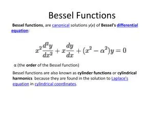
Code Basics • We want a model of the form: • c0*J0(A0*x) + c1*J1(A1*x) + … + c9*J9(A9*x) + F • 21 total constants: c0 – c9, A0 – A9, F • Restrictions: constants less than or equal to one. • So we must find the correct 21 constants! How?
The Loop • Steps: • Define all different combinations of Bessel Functions at 0.1 step sizes for coefficients • Take first combination and find intensity for all residual x-points in data • Find the difference between each residual intensity and square value
The Loop • Steps (cont): • Add all differences up and that gives total difference (or error) for Bessel function with those coefficients • Repeat for all combinations of Bessel Functions • Bessel function with the smallest difference is the best fit of the data
Problem • The number of calculations done is the number of steps for each coefficient to the power of the number of coefficients. • number of steps for each coefficient = 10 • number of coefficients = 21 • Number of calculations = 10^21
Problem • How long does that take to calculate? • 10^5 calculations = 20 minutes • So: • (10^5)/(10^21) = (20 min)/time • So time = 20*10^16 minutes • Or time = 380,517,503,805.2 years • What does this mean?
Solution… maybe • Loop functions seperately: • c0, A, F 6. c5, G, F • c1, B, F 7. c6, H, F • c2, C, F 8. c7, I, F • c3, D, F 9. c8, K, F • c4, E, F 10. c9, L, F
Solution… maybe • Each loop now has 10^3 calculations and takes about 2 seconds. • This gives a nice fit in about 20 seconds. • We can redo this same process starting with the new coefficients and refine the fit.
Possible Problem • Finding Local Minimum instead of Global Minimum
Future • Adding code for fitting at finer resolutions • Completely restarting if this turns out to just be a local minimum.