Download
1 / 40
400 likes | 661 Views
Mid-Term Exam. Next Wednesday Perceptrons Decision Trees SVMs Computational Learning Theory In class, closed book. PAC Learnability. Consider a concept class C defined over an instance space X (containing instances of length n ),

E N D
Mid-Term Exam • Next Wednesday • Perceptrons • Decision Trees • SVMs • Computational Learning Theory • In class, closed book CS446-Spring 06
PAC Learnability • Consider a concept class C • defined over an instance space X (containing instances of length n), • and a learner L using a hypothesis space H. • C is PAC learnable by L using H if • for all f C, • for any distribution D over X, and fixed 0< , < 1, • L, given a collection of m examples sampled independently according to • the distributionD produces • with probability at least(1- ) a hypothesis h H witherror at most • (ErrorD = PrD[f(x) : = h(x)]) • where m is polynomial in 1/ , 1/ , n and size(C) • C is efficiently learnable if L can produce the hypothesis • in time polynomial in 1/ , 1/ , n and size(C) CS446-Spring 06
Occam’s Razor (1) We want this probability to be smaller than , that is: |H|(1-) < ln(|H|) + m ln(1-) < ln() (with e-x = 1-x+x2/2+…; e-x > 1-x; ln (1- ) < - ; gives a safer ) (gross over estimate) It is called Occam’s razor, because it indicates a preference towards small hypothesis spaces What kind of hypothesis spaces do we want ? Large ? Small ? m CS446-Spring 06
K-CNF • Occam Algorithm for f k-CNF • Draw a sample D of size m • Find a hypothesis h that is consistent with all the examples in D • Determine sample complexity: • Due to the sample complexity result h is guaranteed to be a PAC hypothesis How do we find the consistent hypothesis h ? CS446-Spring 06
K-CNF How do we find the consistent hypothesis h ? • Define a new set of features (literals), one for each clause of size k • Use the algorithm for learning monotone conjunctions, • over the new set of literals Example: n=4, k=2; monotone k-CNF Original examples: (0000,l) (1010,l) (1110,l) (1111,l) New examples: (000000,l) (111101,l) (111111,l) (111111,l) CS446-Spring 06
More Examples Unbiased learning: Consider the hypothesis space of all Boolean functions on n features. There are different functions, and the bound is therefore exponential in n. The bound is not tight so this is NOT a proof; but it is possible to prove exponential growth k-CNF: Conjunctions of any number of clauses where each disjunctive clause has at most k literals. k-clause-CNF: Conjunctions of at most k disjunctive clauses. k-term-DNF: Disjunctions of at most k conjunctive terms. CS446-Spring 06
Computational Complexity • However, determining whether there is a 2-term DNF • consistent with a set of training data is NP-Hard CS446-Spring 06
Computational Complexity • However, determining whether there is a 2-term DNF • consistent with a set of training data is NP-Hard • Therefore the class of k-term-DNF is not efficiently (properly) PAC learnable • due to computational complexity CS446-Spring 06
Computational Complexity • However, determining whether there is a 2-term DNF • consistent with a set of training data is NP-Hard • Therefore the class of k-term-DNF is not efficiently (properly) PAC learnable • due to computational complexity • We have seen an algorithm for learning k-CNF. • And, k-CNF is a superset of k-term-DNF • (That is, every k-term-DNF can be written as a k-CNF) CS446-Spring 06
Computational Complexity • However, determining whether there is a 2-term DNF • consistent with a set of training data is NP-Hard • Therefore the class of k-term-DNF is not efficiently (properly) PAC learnable • due to computational complexity • We have seen an algorithm for learning k-CNF. • And, k-CNF is a superset of k-term-DNF • (That is, every k-term-DNF can be written as a k-CNF) • Therefore, C=k-term-DNF can be learned as using H=k-CNF as the hypothesis Space CS446-Spring 06
Computational Complexity • However, determining whether there is a 2-term DNF • consistent with a set of training data is NP-Hard • Therefore the class of k-term-DNF is not efficiently (properly) PAC learnable • due to computational complexity • We have seen an algorithm for learning k-CNF. • And, k-CNF is a superset of k-term-DNF • (That is, every k-term-DNF can be written as a k-CNF) • Therefore, C=k-term-DNF can be learned as using H=k-CNF as the hypothesis Space C H Importance of representation: Concepts that cannot be learned using one representation can sometimes be learned using another (more expressive) representation. Attractiveness of k-term-DNF for human concepts CS446-Spring 06
Negative Results - Examples • Two types of nonlearnability results: • Complexity Theoretic • Showing that various concepts classes cannot be learned, based on • well-accepted assumptions from computational complexity theory. • E.g. : C cannot be learned unless P=NP • Information Theoretic • The concept class is sufficiently rich that a polynomial number of examples • may not be sufficient to distinguish a particular target concept. • Both type involve “representation dependent” arguments. • The proof shows that a given class cannot be learned by algorithms using • hypotheses from the same class. (So?) • Usually proofs are for EXACT learning, but apply for the distribution free case. CS446-Spring 06
Negative Results For Learning • Complexity Theoretic • k-term DNF, for k>1 (k-clause CNF, k>1) • “read-once” Boolean formulas • Quantified conjunctive concepts • Information Theoretic • DNF Formulas; CNF Formulas • Deterministic Finite Automata • Context Free Grammars CS446-Spring 06
Agnostic Learning • Assume we are trying to learn a concept f using hypotheses in H, but f H CS446-Spring 06
Agnostic Learning • Assume we are trying to learn a concept f using hypotheses in H, but f H • In this case, our goal should be to find a hypothesish H, with a minimal training error: CS446-Spring 06
Agnostic Learning • Assume we are trying to learn a concept f using hypotheses in H, but f H • In this case, our goal should be to find a hypothesish H, with a minimal training error: • We want a guarantee that a hypothesis with a good training error will • have similar accuracy on unseen examples CS446-Spring 06
Agnostic Learning • Assume we are trying to learn a concept f using hypotheses in H, but f H • In this case, our goal should be to find a hypothesish H, with a minimal training error: • We want a guarantee that a hypothesis with a good training error will • have similar accuracy on unseen examples • Hoeffding bounds characterize the deviation between the true probability of • some event and its observed frequency over m independent trials. • (p is the underlying probability of the binary variable being 1) CS446-Spring 06
Agnostic Learning • Therefore, the probability that an element in H will have training error • which is off by more than can be bounded as follows: • Using the union bound as before, with=|H|exp{2m2} • we get a generalization bound – a bound on how much will the true error • deviate from the observed error. • For any distribution D generating training and test instance, • with probability at least 1- over the choice of the training set of size m, • (drawn IID), for all hH CS446-Spring 06
Agnostic Learning • An agnostic learner which makes no commitment to whether f is inH • and returns the hypothesis with least training error over at least the • following number of examples can guarantee with probability at least (1-) • that its training error is not off by more than from the true error. • Learnability still depends on the log of the size of the hypothesis space • Previously (with f in H): CS446-Spring 06
Learning Rectangles • Assume the target concept is an axis parallel rectangle Y X CS446-Spring 06
Learning Rectangles • Assume the target concept is an axis parallel rectangle Y + + - X CS446-Spring 06
Learning Rectangles • Assume the target concept is an axis parallel rectangle Y + + - X CS446-Spring 06
Learning Rectangles • Assume the target concept is an axis parallel rectangle Y + + - + + X CS446-Spring 06
Learning Rectangles • Assume the target concept is an axis parallel rectangle Y + + - + + X CS446-Spring 06
Learning Rectangles • Assume the target concept is an axis parallel rectangle Y + + + + - + + + + + + X CS446-Spring 06
Learning Rectangles • Assume the target concept is an axis parallel rectangle Y + + + + + - + + + + + + X CS446-Spring 06
Learning Rectangles • Assume the target concept is an axis parallel rectangle Y + + + + + - + + + + + + X Will we be able to learn the target rectangle? Some close approximation? Some low-loss approximation? CS446-Spring 06
Infinite Hypothesis Space • The previous analysis was restricted to finite hypothesis spaces • Bounds used size to limit expressiveness • Some infinite hypothesis spaces are more expressive than others • E.g., Rectangles, vs. 17- sides convex polygons vs. general convex polygons • Linear threshold function vs. a conjunction of LTUs • Need a measure of the expressiveness of an infinite hypothesis space other • than its size • The Vapnik-Chervonenkis dimension (VC dimension) provides such • a measure • Analogous to |H|, there are bound for sample complexity using VC(H) CS446-Spring 06
Shattering CS446-Spring 06
Shattering CS446-Spring 06
Shattering CS446-Spring 06
Shattering • We say that a set S of examplesis shattered by a set of functions H if • for every partition of the examples in S into positive and negative examples • there is a function in H that gives exactly these labels to the examples • (Intuition: A richer set of functions shatters larger sets of points) CS446-Spring 06
Shattering • We say that a set S of examplesis shattered by a set of functions H if • for every partition of the examples in S into positive and negative examples • there is a function in H that gives exactly these labels to the examples • (Intuition: A richer set of functions shatters larger sets of points) • Left bounded intervals on the real axis:[0,a), for some real number a>0 + + + + + - - a 0 CS446-Spring 06
- + Shattering • We say that a set S of examplesis shattered by a set of functions H if • for every partition of the examples in S into positive and negative examples • there is a function in H that gives exactly these labels to the examples • (Intuition: A richer set of functions shatters larger sets of points) • Left bounded intervals on the real axis:[0,a), for some real number a>0 • Sets of two points cannot be shattered • (we mean: given two points, you can label them in such a way that • no concept in this class that will be consistent with their labeling) + + + + + - + + + + + - - a a 0 0 CS446-Spring 06
Shattering • We say that a set S of examplesis shattered by a set of functions H if • for every partition of the examples in S into positive and negative examples • there is a function in H that gives exactly these labels to the examples • Intervals on the real axis:[a,b], for some real numbers b>a This is the set of functions (concept class) considered here - - + + + + + - - b a CS446-Spring 06
Shattering • We say that a set S of examplesis shattered by a set of functions H if • for every partition of the examples in S into positive and negative examples • there is a function in H that gives exactly these labels to the examples • Intervals on the real axis:[a,b], for some real numbers b>a • All sets of one or two points can be shattered • but sets of three points cannot be shattered - - - - + + + + + - + + + + + - - b b + - + b a CS446-Spring 06
Shattering • We say that a set S of examplesis shattered by a set of functions H if • for every partition of the examples in S into positive and negative examples • there is a function in H that gives exactly these labels to the examples • Half-spaces in the plane: + + + - - - + - CS446-Spring 06
Shattering • We say that a set S of examplesis shattered by a set of functions H if • for every partition of the examples in S into positive and negative examples • there is a function in H that gives exactly these labels to the examples • Half-spaces in the plane: • sets of one, two or three points can be shattered • but there is no set of four points that can be shattered + + + + - - - - + - - + CS446-Spring 06
VC Dimension • An unbiased hypothesis space H shatters the entire instance space X, i.e, • it is able to induce every possible partition on the set of all possible instances. • The larger the subset X that can be shattered, the more expressive a • hypothesis space is, i.e., the less biased. CS446-Spring 06
VC Dimension • We say that a set S of examplesis shattered by a set of functions H if • for every partition of the examples in S into positive and negative examples • there is a function in H that gives exactly these labels to the examples • The VC dimension of hypothesis space H over instance space X • is the size of the largest finite subset of X that is shattered by H. • If there exists a subset of size d can be shattered, then VC(H) >=d • If no subset of sizedcan be shattered, then VC(H) < d • VC(Half intervals) = 1 (no subset of size 2 can be shattered) • VC( Intervals) = 2 (no subset of size 3 can be shattered) • VC(Half-spaces in the plane) = 3 (no subset of size 4 can be shattered) CS446-Spring 06