Download
1 / 52
580 likes | 814 Views
Ch 6 Solar Wind Interactions. Earth’s Magnetic Field. Geomagnetism. Paleomagnetism External Current Systems Sq and L Disturbance Variations Kp, Ap, Dst. Dipole Magnetic Field Geomagnetic Coordinates B-L Coordinate system L-Shells. GEOMAGNETISM.

E N D
Ch 6 Solar Wind Interactions.Earth’s Magnetic Field UML_reinisch_85.511_Ch7
Geomagnetism Paleomagnetism External Current Systems Sq and L Disturbance Variations Kp, Ap, Dst Dipole Magnetic Field Geomagnetic Coordinates B-L Coordinate system L-Shells UML_reinisch_85.511_Ch7
GEOMAGNETISM According to Ampere’s Law, magnetic fields are produced by electric currents: Earth's magnetic field is generated by movements of a conducting "liquid" core, much in the same fashion as a solenoid. The term "dynamo" or “Geodynamo” is used to refer to this process, whereby mechanical motions of the core materials are converted into electrical currents. UML_reinisch_85.511_Ch7
The core motions are induced and controlled by • convection and rotation (Coriolis force). However, • the relative importance of the various possible driving • forces for the convection remains unknown: • heating by decay of radioactive elements • latent heat release as the core solidifies • loss of gravitational energy as metals solidify and migrate • inward and lighter materials migrate to outer reaches of • liquid core. Venus does not have a significant magnetic field although its core iron content is thought to be similar to that of the Earth. Venus's rotation period of 243 Earth days is just too slow to produce the dynamo effect. Mars may once have had a dynamo field, but now its most prominent magnetic characteristic centers around the magnetic anomalies in Its Southern Hemisphere (see following slides). UML_reinisch_85.511_Ch7
The main dipole field of the earth is thought to arise from a single main two-dimensional circulation. • Non-dipole regional anomalies (deviations from the main field) are thought to arise from various eddy motions in the outer layer of the liquid core (below the mantle). • Anomalies of lesser geographical extent (surface anomalies) are field irregularities caused by deposits of ferromagnetic materials in the crust. [The largest is the Kursk anomaly, 400 km south of Moscow]. UML_reinisch_85.511_Ch7
Note on ELECTRIC and MAGNETIC DIPOLES An electrostatic dipole consists of closely-spaced positive and negative point charges, and the resulting electrostatic field is related to the electrostatic potential as follows: By analogy, if we consider the magnetic field due to a current loop, the mathematical form for the magnetic field looks just like that for the electric field, hence the "magnetic dipole" analogy: UML_reinisch_85.511_Ch7
The magnetic field at the surface of the earth is determined mostly by internal currents with some smaller contribution due to external currents flowing in the ionosphere and magnetosphere In the current-free zone Therefore Combined with another Maxwell equation: Yields Laplace’s Equation UML_reinisch_85.511_Ch7
The magnetic scalar potential V can be written as a spherical harmonic expansion in terms of the Schmidt function, a particular normalized form of Legendre Polynomial: internal sources external sources r = radial distance = colatitude = east longitude a = radius of earth (geographic polar coordinates) = 0 for m > n n = 1 --> dipole n = 2 --> quadrapole UML_reinisch_85.511_Ch7
Standard Components and Conventions Relating to the Terrestrial Magnetic Field “magnetic elements” (H, D, Z) (F, I, D) (X, Y, Z) UML_reinisch_85.511_Ch7
Surface Magnetic Field Magnitude (g) IGRF 1980.0 .61 G Max .33 G Min .24 G .67 G UML_reinisch_85.511_Ch7
Surface Magnetic Field H-Component (g) IGRF 1980.0 .025 G .40 G .33 G .13 G .025 G UML_reinisch_85.511_Ch7
Surface Magnetic Field Vertical Component IGRF 1980.0 .61 G 0.0 G 0.0 G 0.0 G .68 G UML_reinisch_85.511_Ch7
Surface Magnetic Field Declination IGRF 1980.0 0° 20° 10° 0° UML_reinisch_85.511_Ch7
Paleomagnetism Natural remnant magnetism (NRM) of some rocks (and archeological samples) is a measure of the geomagnetic field at the time of their production. Most reliable -- thermo-remnant magnetization -- locked into sample by cooling after formation at high temperature (i.e., kilns, hearths, lava). Over the past 500 million years, the field has undergone reversals, the last one occurring about 1 million years ago. See following figures for some measurements of long-term change in the earth's magnetic field. UML_reinisch_85.511_Ch7
Equatorial field intensity in recent millenia, as deduced from measurements on archeological samples and recent observatory data. ~10 nT/year UML_reinisch_85.511_Ch7
The B-L Coordinate System: Curves of Constant B and L The curves shown here are the intersection of a magnetic meridian plane with surfaces of constant B and constant L (The difference between the actual field and a dipole field cannot be seen in a figure of this scale. l UML_reinisch_85.511_Ch7
External Current Systems Currents flowing in the ionosphere and magnetosphere also induce magnetic field variations on the ground. These field variations generally fall into the categories of "quiet" and "disturbed". We will discuss the quiet field variations first. The solar quiet daily variation (Sq) results principally from currents flowing in the electrically-conducting E-layer of the ionosphere. Sq consists of 2 parts: due to the dynamo action of tidal winds; and due to current exhange between the high-latitude ionosphere and the magnetosphere along field lines (see following figure). UML_reinisch_85.511_Ch7
dawn dusk UML_reinisch_85.511_Ch7
Solar Quiet Current systems 10,000 A between current density contours UML_reinisch_85.511_Ch7
DISTURBANCE VARIATIONS In addition to Sq and L variations, the geomagnetic field often undergoes irregular or disturbance variations connected with solar disturbances. Severe magnetic disturbances are calledmagnetic storms. Storms often begin with asudden storm commencement (SSC),after which a repeatable pattern of behavior ensues. However, many storms start gradually (no SSC), and sometimes an impulsive change (sudden impulse or SI) occurs, and no storm ensues. disturbed value of a magnetic element (X, Y, H, etc.): disturbed field X = Xobs - Xq =Dst() + DS() t=t’ longitude Disturbance local time inequality (“snapshot” of the X variation with longitude at a particular latitude) storm-time variation, the average of X around a circle of constant latitude t = storm time, time lapsed from SSC UML_reinisch_85.511_Ch7
Typical Magnetic Storm SSC followed by an "initial" or "positive" phase lasting a few hours. During this phase the geomagnetic field is compressed on the dayside by the solar wind, causing a magnetopause current to flow that is reflected in Dst(H) > 0. During the main phase Dst(H) < 0 and the field remains depressed for a day or two. The Dst(H) < 0 is due to a "westward ring current" around the earth, reaching its maximum value about 24 hours after SSC. During recovery phase after ~24 hours, Dst slowly returns to ~0 (time scale ~ 24 hours). UML_reinisch_85.511_Ch7
Various indices of activity have been defined to describe the degree of magnetic variability. For any station, the range (highest and lowest deviation from regular daily variation) of X, Y, Z, H, etc. is measured (after Sq and L are removed); the greatest of these is called the "amplitude" for a given station during a 3-hour period. The average of these values for 12 selected observatories is the ap index. The Kp index is the quasi-logarithmic equivalent of the ap index. The conversion is as follows: The daily Ap index, for a given day, is defined as UML_reinisch_85.511_Ch7
Ap and Solar Cycle Variation • Long-term records of annual sunspot numbers (yellow) show clearly • the ~11 year solar activity cycle • The planetary magnetic activity index Ap (red) shows the occurrence • of days with Ap • ≥ 40 UML_reinisch_85.511_Ch7
Transformer Heating Saturation of the transformer core produces extra eddy currents in the transformer core and structural supports which heat the transformer. The large thermal mass of a high voltage power transformer means that this heating produces a negligible change in the overall transformer temperature. However,localised hot spots can occur and cause damage to the transformer windings UML_reinisch_85.511_Ch7
How Geomagnetic Variations Affect Pipelines Time-varying magnetic fields induce time-varying electric currents in conductors. Variations of the Earth's magnetic field induce electric currents in long conducting pipelines and surrounding soil. These time varying currents, named "telluric currents" in the pipeline industry, create voltage swings in the pipeline-cathodic protection rectifier system and make it difficult to maintain pipe-to-soil potential in the safe region. During magnetic storms, these variations can be large enough to keep a pipeline in the unprotected region for some time,which can reduce the lifetime of the pipeline. See example for the 6-7 April 2000 geomagnetic storm on the following page. UML_reinisch_85.511_Ch7
7.3 Ionospheres • THE NEUTRAL ATMOSPHERE • Temperature and density structure • Hydrogen escape • Thermospheric • variations and • satellite drag • Mean wind structure UML_reinisch_85.511_Ch7
Tropo (Greek: tropos); “change” Lots of weather Strato (Latin: stratum); Layered Meso (Greek: messos); Middle Thermo (Greek: thermes); Heat Exo (greek: exo); outside UML_reinisch_85.511_Ch7
Variation of the density in an atmosphere with constant temperature (750 K). UML_reinisch_85.511_Ch7
Vertical distribution of density and temperature for high solar activity (F10.7 = 250) at noon (1) and midnight (2), and for low solar activity (F10.7 = 75) at noon (3) and midnight (4) according to the COSPAR International Reference Atmosphere (CIRA) 1965. UML_reinisch_85.511_Ch7
Atmospheric Compositions Compared The atmospheres of Earth, Venus and Mars contain many of the same gases, but in very different absolute and relative abundances. Some values are lower limits only, reflecting the past escape of gas to space and other factors. UML_reinisch_85.511_Ch7
Average Temperature Profiles for Earth, Mars & Venus Venus night day Venus Mars Earth UML_reinisch_85.511_Ch7
At 80-100 km, the time constant for mixing is more efficient than recombination, so mixing due to turbulence and other dynamical processes must be taken into account (i.e., photochemical equilibrium does not hold). Mixing transports O down to lower (denser) levels where recomb- ination proceeds rapidly (the "sink" for O). After the O recombines to produce O2, the O2 is transported upward by turbulent diffusion to be photodissociated once again (the "source" for O). O Concentration UML_reinisch_85.511_Ch7
The most variable parts of the solar spectrum are absorbed above about 100 km UML_reinisch_85.511_Ch7
Formation of Ionospheres UML_reinisch_85.511_Ch7
HYDROSTATIC EQUILIBRIUM If ….. n = # molecules per unit volume m = mass of each particle nm dh = total mass contained in a cylinder of air (of unit cross-sectional area) Then, the force due to gravity on the cylindrical mass = g nmdh and the difference in pressure between the lower and upper faces of the cylinder balances the above force in an equilibrium situation: P + dP dP P nmgdh UML_reinisch_85.511_Ch7
Assuming the ideal gas law holds, Then the previous expression may be written: where H is called the scale height and UML_reinisch_85.511_Ch7
This is the so-called hydrostatic law or barometric law. Integrating, where and z is referred to as the "reduced height" and the subscript zero refers to a reference height at h=0. Similarly, For an isothermal atmosphere, then, UML_reinisch_85.511_Ch7