Download
1 / 78
780 likes | 799 Views
Firewall Design: Consistency, Completeness, and Compactness. Authors: Mohamed G. Gouda and Xing-Yang Alex Liu Presenters: Jonathan Fomby and Matthew Ginley. Firewall Basics. Placed at the entrance (borders) of private networks Examine all traffic passing through (source IP, dest IP, etc.)

E N D
Firewall Design: Consistency, Completeness, and Compactness Authors: Mohamed G. Gouda and Xing-Yang Alex Liu Presenters: Jonathan Fomby and Matthew Ginley
Firewall Basics • Placed at the entrance (borders) of private networks • Examine all traffic passing through (source IP, dest IP, etc.) • Accept, Discard, Log, Reply, Re-route, etc. as appropriate • Implemented as additional software or stand-alone hardware (appliance) • Functionally the same as packet filter or packet classifier, yet firewall implies security
Firewall as a Set of Rules • Firewall functionality can be represented as an ordered list of rules • Rule format • Traditionally displayed as a table, but this paper uses individual Boolean formulas • <predicate> <decision> • authors only consider accept and discard decisions • predicate is Boolean expression over packet fields
Firewall – As a List of Rules ( I=0 ^ S=any ^ D=s ^ P=tcp ^ T=25 a, I=0 ^ S=any ^ D=s ^ P=any ^ T=any d, I=0 ^ S=m ^ D=any ^ P=any ^ T=any d, I=1 ^ S=h ^ D=any ^ P=any ^ T=any a, I=1 ^ S=any ^ D=any ^ P=any ^ T=any a ) An ordered listing of Boolean expressions
Firewall Operation • Rules are compared individually against a packet • Rules compared according to a specified order (i.e. importance) • The first rule to match is chosen and followed • Usually a final catch-all rule (probably discard)
Firewalls – Stateful Packet Filters (text p.629) • traditional packet filters do not examine higher layer context • i.e. matching return packets with outgoing flow • stateful packet filters address this need • they examine each IP packet in context • keep track of client-server sessions • check each packet validly belongs to one • hence are better able to detect bogus packets out of context
Note of Limitation • The authors do not discuss state considerations • By adding state fields to packet fields, this should be feasible • When filtering packets, check these fields in addition to packet fields
3 C’s • Consistency: correct ordering of rules • Completeness: every packet satisfies at least one rule • Compactness: no redundant rules
SIMPLE** Firewall Example • Accept incoming SMTP packets on Int0 destined for Mail Server • Accept all outgoing packets
Packet Fields • I – incoming interface on the firewall • S – original source • D – final destination • P – transport protocol used • T – destination port • Many others not used by authors: source port, packet flags (IP, TCP, others), application layer message, etc.
Continuing the Example • Accept incoming SMTP packets on Int0 destined for Mail Server • (I = 0) ^ (S = any) ^ (D = MailServer) ^ (P = TCP) ^ (T = 25) Accept • Discard incoming non-SMTP packets on Int0 destined for Mail Server • (I = 0) ^ (S = any) ^ (D = MailServer) ^ (P = any) ^ (T = any) Discard
Cont. • Discard incoming packets whose source is a Malicious Host • (I = 0) ^ (S = MH) ^ (D = any) ^ (P = any) ^ (T = any) Discard • Accept outgoing HTTP packets from any non-server host h • (I = 1) ^ (S = h) ^ (D = any) ^ (P = TCP) ^ (T = 80) Accept • Accept all outgoing packets • (I = 1) ^ (S = any) ^ (D = any) ^ (P = any) ^ (T = any) Accept
Problems with Example Rules • Consistency Error • Rules 1 and 3 can be matched to the same packet, yet have conflicting decisions • Rule 1 will always be applied, thus ignoring the discarding of malicious packets intended by Rule 3 • Solution: Place Rule 3 first
Problems Cont. • Completeness Error • Packets with (I=0 ^ S≠MH ^ D≠MailServer) do not satisfy any rules • Solution: add the following rule (at the end of list): (I = 0) ^ (S = any) ^ (D = any) ^ (P = any) ^ (T = any) Accept
Problems Cont. • Compactness Error • Rule 4 is redundant • All packets matching rule 4 will match rule 5 as well, with both rules accepting • Solution: remove Rule 4
Our Focus • “… a method for designing the sequence of rules of a firewall to be consistent, complete, and compact.” • Start with a firewall decision diagram (defined later) that is processed by a series of algorithms • Resulting FDD is functionally equivalent, yet consistent, complete, and compact
Algorithm Summary • Starting with a user specified FDD f • #1 – FDD Reduction • Output: a reduced FDD equivalent to f • #2 – FDD Marking • Output: an equivalent, marked version f’ of f
Algorithm Summary • #3 – Firewall Generation • A firewall r over the same fields as f’, that is functionally equivalent to f’ and each rule in r is provided a rank • #4 – Firewall Compaction • Output: a compact firewall, equivalent to r • #5 – Firewall Simplification • Output: a simple firewall, equivalent to r
Related Work • [3] : Existing Design Errors • Efficient Data Structures for Rule Checking • [12] : Trie Data Structures • [6] : Area Based Quadtrees • [8] : Fat Inverted Segment Trees • [9] : Survey of such data structures • Specification Languages • [3] : Simple Model Definition Language • [10] : Lisp-like specification language • [4] : Declarative Predicate Language • [1] : High level firewall language
More Related Work – Detecting Conflicting Rules • [11] : Detecting and Resolving Packet Filter Conflicts • Ambiguity in packet classification deserves more attention • Demonstrates resolving conflicts by prioritization is ineffective • Resolve conflicts by adding filters
More Related Work – Detecting Conflicting Rules • [7] : Internet packet filter management and rectangle geometry • Claim that previous best for detecting conflicts was O(n2 log n) time • Their presented approach is O(n3/2) • Based on rectangle coverage of a kD-tree and stripe conflict detection (lots of difficult theory)
More Related Work – Detecting Conflicting Rules • [2] : Fast and scalable conflict detection for packet classifiers • Claim the best known algorithm for conflict detection is naïve comparison, O(n2) • Their approach is based on the aggregation of bit vector data • Do not provide theoretical complexity, but state “a factor of 40 improvement for a 20,000 rule database”
More Related Work – Decision Diagrams • [5] : Binary Decision Diagrams • [13] : Interval Decision Diagrams • Similar to Firewall Decision Diagrams, but the diagram format is not the focus (nor particularly novel)
Firewall Decision Diagrams • Circles are non-terminal nodes • Boxes are terminal nodes (always ‘a’ = Accept or ‘d’ = Discard for our purposes • Arrows are edges • Decision Path: directed path from the root to a terminal node
Fields • field Fi: variable whose value is taken from the domain of Fi • Domain of Fi, D(Fi): a predefined interval of nonnegative integers • Packet over fields F0,…, Fn-1: an n-tuple (p0,…, pn-1) where each pi is taken from the corresponding domain and field
Firewall Decision Diagram An FDD f over the fields F0,…, Fn-1 IS • Acyclic and directed graph • Satisfies the following 5 properties • f has a root and 2 or more terminal nodes (leaves) • each non-terminal node v is labeled with one of the above fields, F(v); a terminal node v is labeled with ‘a’ or ‘d’ • No two nodes on a decision path have the same label
Firewall Decision Diagram • Each edge e leaving node v is labeled with an integer set I(e) (a subset of D(F(v))) • For any non-terminal node v, the set E(v) of all edges leaving v must satisfy: • Consistency: any distinct ei and ek in E(v), I(ei) ∩ I(ek) = empty set • Completeness: Ue єE(v)I(e) = D(F(v))
Firewall Decision Diagrams • This FDD is over fields F0, F1 • Domain of all fields is [0, 9] • one possible decision path: F0є [4,5] ^ F1є [2,3] U [5,7] a • In a decision path, there is 0 or 1 Boolean primitive for each field of the FDD (0 implies any value for that field).
Firewall Decision Diagrams • FDDs are represented as a sequence of rules, each of the form • F0є S0 ^ … ^ Fn-1є Sn-1 <decision> • 1 to 1 correspondence of decision paths in the FDD to rules • Order does not matter (later changes) • Firewall: sequence of rules that represents an FDD
Acceptance and Discarding • For a packet (p0,…, pn-1) over fields F0,…,Fn-1 received by an FDD f over the same fields • Accepted: iff f has an accepting rule such that p0є S0 ^ … ^ pn-1 є Sn-1 holds • Discarded: iff f has a discarding rule such that ↑ • For the set of all packets, Σ • f.accept: the subset of Σ that contains all packets accepted by f • f.discard: the subset of Σ that contains all packets discarded by f
Acceptance and Discarding • FDD Equivalence: FDDs f and g over the same fields are equivalent iff • f.accept = g.accept and • f.discard = g.discard • Thm. 1: for any FDD f over fields F0,…,Fn-1 • f.accept ∩ f.discard = empty set • f.accept U f.discard = Σ
FDD Reductions • Advantageous to reduce # of decision paths without changing accept and discard sets • Auxiliary Def.--Isomorphic Nodes. Two nodes, v0 and v1, are isomorphic iff (1) or (2) is satisfied. • (1) v0 and v1 Are terminal nodes with the same label • (2) v0 and v1 are non-terminal nodes with an 1-to-1 correspondence between the outgoing edges of v0 and outgoing edges of v1
Isomorphic Node Example • The above red-highlighted nodes are isomorphic • Same label: F1 • 2 edges: one edge with label [2,3] U [5,7] incoming on ‘a’, and one edge with label [0,1] U [4,4] U [8,9] incoming on ‘d’
FDD Reductions • An FDD f is called reducediff it satisfies the following three conditions: • 1. f has no node with exactly one outgoing edge. • 2. f has no two edges that are outgoing of one node and are incoming of another node. • 3. f has no two distinct isomorphic nodes.
Algorithm 1: FDD Reduction • Input: an FDD f • Output: a reduced FDD that is equivalent to f • Repeat steps 1-3 until none can be applied further • 1. If f has a node v0 with only one outgoing edge e and if e is incoming of another node v1, then remove v0 and e from f and make the incoming edges of v0 incoming of v1.
Algorithm 1 • 2. If f has two edges e0 and e1 that are outgoing of node v0 and incoming of node v1, then remove e0 and make the label of e1 be the integer set I(e0) U I(e1),where I(e0) and I(e1) are the integer sets that labeled edges e0 and e1 respectively. • 3. If f has two isomorphic nodes v0 and v1, then remove node v1 and its outgoing edges, and make the incoming edges of v1 incoming of v0.
Marking of FDDs • A “Marked” FDD is similar to the reduced FDD, with an “ALL” label being added to a single edge from each node • The number of simple rules eventually generated in the firewall depends upon the “degree” of a marked FDD • Nodes and Edges are given degrees in order to find which edges should be marked ALL
Marking of FDDs (cont.) • Many marked versions of reduced FDDs are possible • Number of simple rules generated by a firewall is determined by the degree of the marked FDD • Note that this refers to the final “simple” rules, not the number of rules that will be generated in the intermediate steps • Degree is determined by which edges are marked ALL • Smaller degree -> Fewer final rules -> Simpler firewall -> Good Thing™
Marking of FDDs (cont.) • Degree of a set of integers, denoted deg(S), is the smallest number of non-overlapping integer intervals that covers set S. • Ex: For the set {0,1,3,4,5,7,9}, the degree is 4, composed of the intervals [0,1], [3,5], [7,7], and [9,9]
Marking of FDDs (cont.) • Degree of an edgee is denoted deg(e) • If e is marked ALL, then deg(e) = 1 • Else, deg(e) = deg(S) Degree 1 Degree 2 Degree 2 Degree 3
Marking of FDDs (cont.) • Degree of a nodev, denoted deg(v), is calculated using a simple formula • If v is a terminal node, then deg(v) = 1 • Else, for a non-terminal node v with k outgoing edges, e0, …, ek-1 that are incoming of nodes v0, …, vk-1 respectively, then deg(v) = ∑ deg(ei) × deg(vi)
Marking of FDDs (cont.) • To put it in simpler terms: The get the degree of a node, take each outgoing edge and multiply its degree by the degree of the node into which the edge leads. Add these together, and you have the degree of the node.
Marking of FDDs (cont.) • Since the edges marked ALL have such a large impact on the complexity of the firewall, it is critical to pick the ALL-edges carefully and minimize the degree of the FDD • One edge from the collection of edges leaving each node is marked ALL, so pick the edge that would minimize the degree of said node to label ALL
Marking of FDDs – Algorithm 2 • Step 1: Compute the degree of each terminal node v in f as deg(v) = 1 • Step 2: For every node v whose degree has not yet been calculated • 1 – Find the outgoing edge e of current node whose quanity (deg(ej)-1) x deg(vj) is larger than or equal to the corresponding quantity in every other outgoing edge of v • 2 – Mark edge ej with ALL • Compute the degree of v with the summation formula
Marking of FDDs (cont.) 3 + 1 = 4 3 + 2 = 5 1 1 2 2+1 = 3 2+1=3 1 1 1 2 2 Terminal Nodes: Degree = 1 Two Marked FDDs from the same Reduced FDD
Firewall Generation • Generated Firewall is a sequence of rules such that each rule corresponds to a decision path in the marked FDD • This step produces the rules of the firewall, as well as a ranking for each rule, and two predicates, the exhibited and the original predicate • Rank is used for ordering the rules, predicates for making the firewall “Compact” in the next step
Firewall Generation (cont.) • For our purposes, a Firewall r over the fields F0,…,Fn-1 is a sequence of rules r0,…,rm-1 where each rule is of the form F0ЄS0Λ … ΛFn-1ЄSn-1 → <decision> where each Si is either the mark ALL or a nonempty set of integers from the domain of field Fi, and the <decision> is either a (accept) or d (discard). Ex. F0Є [4,7] ΛF1Є [2,3] U [5,7] → a