Download
1 / 34
360 likes | 505 Views
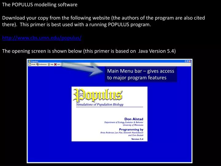
The POPULUS modelling software Download your copy from the following website (the authors of the program are also cited there). This primer is best used with a running POPULUS program. http://www.cbs.umn.edu/populus/ The opening screen is shown below (this primer is based on Java Version 5.4).

E N D
The POPULUS modelling software Download your copy from the following website (the authors of the program are also cited there). This primer is best used with a running POPULUS program. http://www.cbs.umn.edu/populus/ The opening screen is shown below (this primer is based on Java Version 5.4) Main Menu bar – gives access to major program features
The POPULUS modelling software Depending on your screen size, you may need to adjust the POPULUS program windows. Each of them can be scaled by clicking-and-dragging on any edge (just like any other window). POPULUS windows may be repositioned by clicking-and-dragging on their heading. POPULUS windows may be scaled by clicking-and-dragging on any edge.
The POPULUS modelling software A Help document can be accessed by clicking on the Help button in the menu bar. The help document is a pdf file and will require a pdf reader.
The POPULUS modelling software Access the models by clicking on the Model button. We’ll discuss Lotka-Volterra competition models in this section. • NOTE: This primer assumes that you have mastered the lesson(s) on: • Density-Independent growth models • Density-Dependent growth models
The POPULUS modelling software: Lotka-Volterra Competition N(0) refers to the initial population abundance of the population prior to the competitive interaction. The model simulates the competitive interaction between two species. Hence, you are given two sets of parameters to define. r is the species’ growth potential (the balance between birth and death rates). K is the carrying capacity of each species (it is the maximum abundance the environment can sustain). Known as competition coefficients, alpha (α) and beta (β) simulates the competitive pressure a species exerts on another. α is the effect of species 2 on 1 while β is the effect of species 1 on 2.
The POPULUS modelling software: Lotka-Volterra Competition There are two plot types available in this model. N vs t graphs the abundance of both populations over time while N2 vs N1 shows the changing abundance of both populations as they compete with each other. We will be using the ‘Run until steady state’ condition throughout. POPULUS will run the simulation until a definitive outcome is reached (both species co-exist or one wins while the other becomes extinct).
The POPULUS modelling software: Lotka-Volterra Competition We will begin our discussion on this model by assuming two species that are duplicates of each other. Input the following parameters and click ‘View’ to see the plot.
The POPULUS modelling software: Lotka-Volterra Competition Let’s look at the basics before analyzing the graph. The y-axis plots the abundance of both species. Stationary phase Log phase Lag phase The x-axis shows the generation time.
The POPULUS modelling software: Lotka-Volterra Competition The model simulates the interaction between two competing species (Red N1 and Blue N2). So how come only the blue line is shown below? This is because the two species are so identical that they grow in exactly the same way. The red line is there- just covered by the blue line. So the graph below shows two equally competitive species. Notice however, that neither of them reached their K (which was set at 500). Think of a family-sized pizza being shared by 5 people. If you can eat 3 slices by yourself (your K = 3), would you still be able to do so when there are 4 other people eating? The K reached by both species is lower than the K they would have reached without competition (when growing alone). The lower K reflects the competitive pressure felt by both species. (Both of them got a lower K- both of them lost). Let’s call this resultant K and it is obtained by projecting the Stationary phase onto the y-axis. In this example, resultant K is ~340 (approximately 340).
The POPULUS modelling software: Lotka-Volterra Competition Close the active graph and click on the N2 vs N1 plot type. Activates the N2 vs N1 plot type. You may also click on this without closing the active graph. (It will automatically change graphs). Closes the active graph.
The POPULUS modelling software: Lotka-Volterra Competition The graph below should be on your POPULUS screen at this time. If vector analysis is done, we can see that all the resultant vectors will point towards the intersection point (the stable point of co-existence). If the white vectors shown below are not clear to you, then you will need to review an earlier lesson on Lotka-Volterra models uploaded in my blog. The stable point of co-existence. This model predicts that the two species can live together. The green line is a vector that traces the result of the competitive interaction. Recall that we started with 10 individuals each of N1 and N2 (open circle). The green line ended (shaded circle) in the point of co-existence.
The POPULUS modelling software: Lotka-Volterra Competition POPULUS lets you simulate numerous starting points for these two species. To do this, you just have to change the initial abundance of each species. Shown below are the parameters used for the upper-right graph in the next slide. Note the entered N(0) values.
The POPULUS modelling software: Lotka-Volterra Competition These graphs show various starting points for the competitive interaction. N1(0) = 900 N2(0) = 400 N1(0) = 10 N2(0) = 800 N1(0) = 50 N2(0) = 200 N1(0) = 800 N2(0) = 100
The POPULUS modelling software: Lotka-Volterra Competition Now let’s model a situation in which the species are not equally competitive. Let us begin by first changing their r. Input the following parameters and choose the N vs t plot type. We have given Species 2 twice the r of Species 1. This means that Sp 2 will grow faster than Sp 1. (Growth here is taken as increase in number and NOT growth in size.)
The POPULUS modelling software: Lotka-Volterra Competition We can see here that since BLUE grows faster (it has higher r), it initially gains the upperhand over RED (encircled area). Eventually, however, both species will settle for a lower resultant K as they reach the point of co-existence. Now let’s look at the N2 vs N1 plot. (The previous N vs t plot is shown as an inset for comparison).
The POPULUS modelling software: Lotka-Volterra Competition The vector plot remains essentially the same.
The POPULUS modelling software: Lotka-Volterra Competition What would happen if they had different K’s? Input the following parameters and choose the N vs t plot type. (Note that we’ve reset their r to equal values.) We have set the K of Species 2 just a little higher than Species 1. This means that the environment can support more individuals of Species 2 than of Species 1. Consider birds and ants. You can easily find 1,000 ants in HEDCen but you will be hardpressed to find even a 100 birds. This is because there is just not enough food, water and space for a 100 birds in our school.
The POPULUS modelling software: Lotka-Volterra Competition Note that both species would still co-exist but Species 2 has achieved a higher resultant K than Species 1. It can be seen in the encircled area that Species 2 reached a resultant K of ~460 while Species 1 reached ~270. The resultant K1 of 270 is lower than the previous resultant K1 (~330) when the two species were equally competitive (see inset plot). This means that although the species are still co-existing, Species 1 is clearly the less competitive species.
The POPULUS modelling software: Lotka-Volterra Competition Will the species still co-exist if their K’s are very different? Let’s create a series of plots as we increase K2 from 500 to 1,000 by increments of 100. Input the given parameters and generate the graphs shown from slide to slide. Use the N vs t plot type.
The POPULUS modelling software: Lotka-Volterra Competition From equal K’s we move to K2 = 600 and K1 = 500. Notice that the resultant K2 is now higher than the resultant K1.
The POPULUS modelling software: Lotka-Volterra Competition Settings: K2 = 700 and K1 = 500.
The POPULUS modelling software: Lotka-Volterra Competition Settings: K2 = 800 and K1 = 500.
The POPULUS modelling software: Lotka-Volterra Competition Settings: K2 = 900 and K1 = 500.
The POPULUS modelling software: Lotka-Volterra Competition Settings: K2 = 1,000 and K1 = 500. At this point, we see that Species 1 has been driven to extinction by Species 2. The curve for Species 1 has touched the x-axis. This happens only when the y-axis, abundance, has reached zero (recall the definition of x-intercept). Click here to see the changes again. Otherwise, click elsewhere to proceed.
The POPULUS modelling software: Lotka-Volterra Competition Next let’s see the changes in the vector plots (N2 vs N1 plot type) as K2 increases. Click anywhere to start the animation. Click here to see the changes again. Otherwise, click elsewhere to proceed.
The POPULUS modelling software: Lotka-Volterra Competition At this point, we have left the model of co-existence and entered the model where one species wins at the expense of the other. This will be discussed in a later release. We can see that the area where Species 1 grows better than Species 2 (encircled) decreases until Species 1 becomes extinct (The green resultant vector touches the y-intercept).
The POPULUS modelling software: Lotka-Volterra Competition Let us now examine the competitive interaction between two species with diferrent coefficients of competition. Input the parameters below. As you can see, Species 2 is a better competitor since it has a lower Beta (β) than the Alpha (α) of Species 1. We have set the β of Species 2 just a little lower than the α of Species 1. Recall that β is the effect of Species1 on Species2 while α is the effect of Species2 on Species 1. So if β is lower than α, this means that Species2 is a stronger competitor than Species1.
The POPULUS modelling software: Lotka-Volterra Competition Will the species still co-exist if their α/β are very different? What follows is a series of plots as we decrease β from 0.5 to 0.1 by increments of 0.1. Input the given parameters and generate the graphs shown from slide to slide. Use the N vs t plot type.
The POPULUS modelling software: Lotka-Volterra Competition α = 0.5; β = 0.4
The POPULUS modelling software: Lotka-Volterra Competition α = 0.5; β = 0.3
The POPULUS modelling software: Lotka-Volterra Competition α = 0.5; β = 0.2
The POPULUS modelling software: Lotka-Volterra Competition α = 0.5; β = 0.1 It becomes evident that the effect of decreasing β is similar to the effect of increasing K2. Biologically speaking, this makes sense since both changes will make Species 2 more competitive than Species 1.
The POPULUS modelling software: Lotka-Volterra Competition Though quite similar, we end our discussion with the presentation of the changes in the vector plots (N2 vs N1 plot type) as β decreases. Click anywhere to start the animation. We can see that the area where Species 1 grows better than Species 2 (encircled) decreases until Species 1 becomes extinct. If β becomes much less than α, then we can predict that Species 1 will be driven to extinction. Recall that this was also observed when K2 was increased.
The POPULUS modelling software: Lotka-Volterra Competition We end our discussion of the Lotka-Volterra Competition models where co-existence is possible. To continue, you must download the other models from the ESIII blog.