Download
1 / 25
250 likes | 271 Views
Explore the theory, structure, and operations of Splay Trees, a self-adjusting binary search tree with advantageous features for data structure performance. Learn about key operations like access, insert, delete, join, and split, supported by efficient restructuring heuristics.

E N D
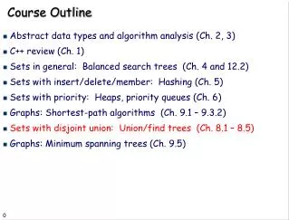
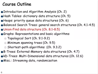
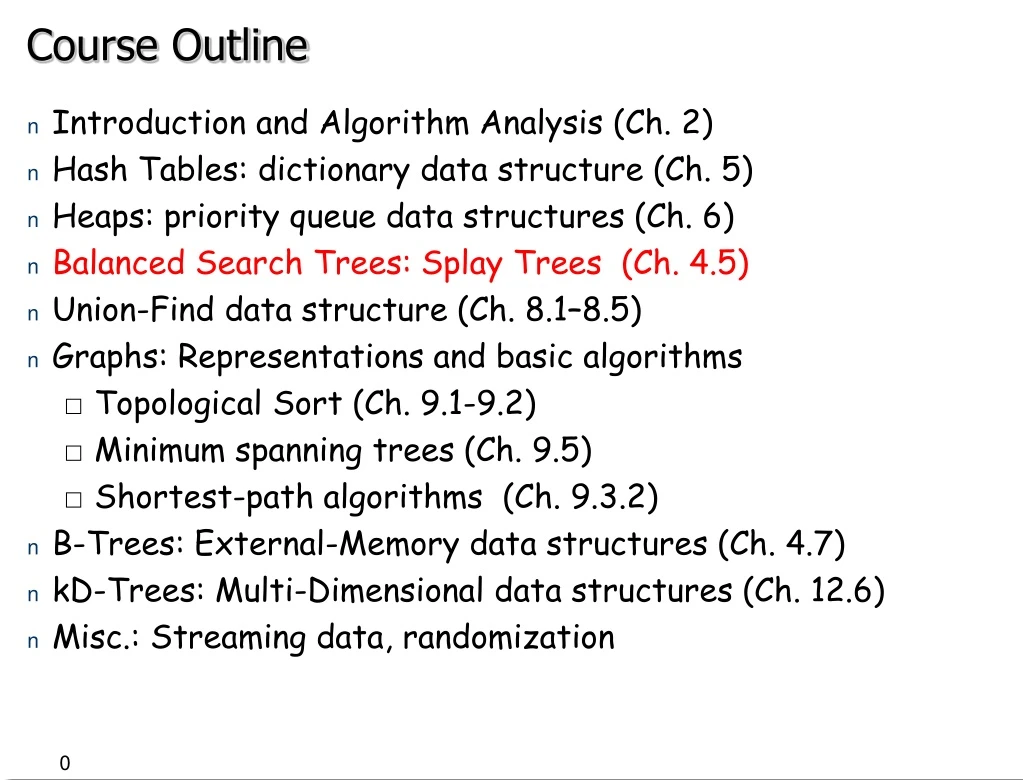
Course Outline • Introduction and Algorithm Analysis (Ch. 2) • Hash Tables: dictionary data structure (Ch. 5) • Heaps: priority queue data structures (Ch. 6) • Balanced Search Trees: Splay Trees (Ch. 4.5) • Union-Find data structure (Ch. 8.1–8.5) • Graphs: Representations and basic algorithms • Topological Sort (Ch. 9.1-9.2) • Minimum spanning trees (Ch. 9.5) • Shortest-path algorithms (Ch. 9.3.2) • B-Trees: External-Memory data structures (Ch. 4.7) • kD-Trees: Multi-Dimensional data structures (Ch. 12.6) • Misc.: Streaming data, randomization
Splay trees • Invented by Sleatorand Tarjan. Self-adjusting Binary Search Trees. JACM, pp. 652-686, 1985. • BSTs (AVL, weight balanced, B-Trees) have • O(log n) worst case search • but are complicated to implementand/or require extra space for balance • No explicit balance condition in Splay Trees • Instead apply a simple restructuring heuristic, called splaying every timethe tree is accessed.
Splay trees: Intuition • For search cost to be small in a BST, the item must be close to the root. • Many tree-restructuring rules try to move the accessed item closer to the root. • Same idea behind caching---keep recently accessed data in fast memory.
Splay trees: Intuition • Two classical heuristics are: • Single rotation: after accessing item i at a node x, rotate the edge joining x to its parent; unless x is the root. • Move to Root: after accessing i at a node x, rotate edges joining x and p(x), and repeat until x becomes the root. • Unfortunately, neither heuristic has O(log n) search cost: • Show arbitrarily long access sequences where time per access is O(n).
Splay trees: Intuition • Sleator-Tarjan's heuristic similar to move-to-front, but its swaps depend on the structure of the tree. • The basic operation is rotation.
Splay trees: Advantages • Simplicity and uniformity • Elegant theory and amortized analysis • average over a Worst-case sequence • useful metric for data structure performance • Besides access, insert, delete, many other useful ops • Access always brings node to the root • Join • Split
Splaying at a Node • To splay at a node x, repeat the following step until x becomes the root: • Case 1 (Zig): [terminating single rotation] if p(x) is the root, rotate the edge between x and p(x); and terminate.
Splaying at a Node • Case 2 (zig-zig): [two single rotations] if (p(x) not root) and (x and p(x) both left or both right children) first rotate the edge from p(x) to its grandparent g(x), and then rotate the edge from x to p(x).
Splaying at a Node • Case 2 (zig-zag): [double rotation] if (p(x) not root) and (x is left child and p(x) right child) first rotate the edge from from x to p(x), and then rotate the edge from x to its new p(x).
Splay trees G X P P G D X A A B C D B C G X P D P A X C G B A B C D • Splayat a node: rotate the node up to the root • Basic operations (repeat until node X is at root): • zig-zag: • zig-zig:
Splay Tree Properties • Fact 1. Splaying at a node x of depth d takes O(d) time. • Fact 2. Splaying moves x to the root, and roughly halves the depth of every node on the access path.
Splay Tree Operations • access (i,t): return a pointer to location of item i, if present; otherwise, return a null pointer. • insert (i,t): insert item i in tree t, if it is not there already; • delete (i,t): delete i from t, assuming it is present. • join (t1, t2): combines t1and t2into a single tree and returns the resulting tree; assume all items in t1smaller than t2 • split (i,t): return two trees: t1, containing all items less than or equal to i, and t2, containing items greater than i. This operation destroys t.
Splay Tree: Implementing the Operations • access (i,t) • Search down from the root, looking for i. • If search reaches a node x containing i, we splay at x and return the pointer to x. • If search reaches a null node, we splay the last non-null node, and return a null pointer.
Insert and Delete in Splay Trees • Insert, delete easily implemented using join and split. • because access(x) moves x to the root. • For join(t1, t2), first access the largest item in t1. • Suppose this item isx. After the access,xis at the root of t1. • Becausexis the largest item in t1, the root must have a null right child. Simply make t2's root to be the right child of t1. • Return the resulting tree. • For split(x,t), first do access(x,t). • If root >x, then break the left child link from the root, and return the two subtrees. • Otherwise, break the right child link from the root, and return the two subtrees. • In all cases, special care if one of subtrees is empty.
Insert in Splay Trees • To do insert(x,t), perform split(x,t). • Replace t with a new tree consisting of a new root node containingx, whose left and right subtreesare t1 and t2returned by the split.
Delete in Splay Trees • To do delete(x,t), perform access(x,t), and then replace t by the join of its left and right subtrees.
Splay trees: the main theorem Starting with an empty tree,any m operations (find, insert, delete)take O(m log n) time,where n is the maximum # of items ever in the tree Lemma: Any sequence of m operations requires at most 4 m log n + 2 splay steps. (The theorem follows immediately from the lemma.)
Splay trees: Main Theorem Starting with an empty tree,any m operations (find, insert, delete)take O(m log n) time,where n is the maximum # of items ever in the tree • Proof: “credit accounting” • just count the cost of splaying • each operation gets 3 lg n + 1 coins • one coin pays for one splay step • each node holds floor(lg(size of subtree)) coins
Splay trees: proving the lemma • Each operation gets 4 log n + 2 coins (3 log n + 1is enough for all but insert ) • One splay step costs one coin, from somewhere • Some of the leftover coins are left “on the tree”to pay for later operations Credit invariant:Every tree node holds log(subtree size) coins (rounded down to an integer)
Splay trees: maintaining the credit invariant G X P P G D X A A B C D B C • lss(x) = log(subtree size) before step; lss’ after step • zig-zag step costs 1 coin (to do the step) plus lss’(x) – lss(x) + lss’(p) – lss(p) + lss’(g) – lss(g)(to maintain the invariant) • this is always <= 3(lss’(x) – lss(x)) [complex argument] • similarly for zig-zig; 1 more for last half step • total cost of splay is <= 3(lss(root))+1 = 3 log n + 1
Splay trees: end of the main proof • maintaining invariant during splay costs <= 3 log n + 1 coins • maintaining invariant during insert may cost an extra log n + 1 coins (because lss goes up) • maintaining credit invariant never costs more than 4 log n + 2 coins • Lemma: Any sequence of m operations requires at most 4 m log n + 2 splay steps. • Theorem: Starting with an empty tree, any m operations (find, insert, delete) take O(m log n) time