Download
1 / 13
130 likes | 280 Views
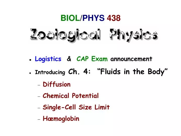
BIOL / PHYS 438. Logistics & CAP Exam announcement Introducing Ch. 4: “Fluids in the Body†Diffusion Chemical Potential Single-Cell Size Limit H æmoglobin. Logistics. Assignment 1 : login, update, Email anytime! Assignment 2 : due Tuesday

E N D
BIOL/PHYS438 • Logistics & CAP Exam announcement • Introducing Ch. 4: “Fluids in the Body” • Diffusion • Chemical Potential • Single-Cell Size Limit • Hæmoglobin
Logistics Assignment 1: login, update, Email anytime! Assignment 2: due Tuesday Assignment 3: Tuesday → Thursday 15 Feb Assignment 4: Thu 15 Feb → Tue after Break Spring Break: 17-25 Feb: work on Project too!
More Logistics • People Database • Please log in, Update your Profile (especially your Email address!) and participate. • Few received my Email notice about the fabulous Harvard video on cellular nanoprocesses. :-( • Projects • Draft proposals due today! • How about a Web Database of Project Ideas? (like the Quips database – anyone can contribute)
Conduction of Heat HOT side (TH) • Q cond = •A•(TH − TC) /ℓ ℓ Thermal conductivity [W•m−1•K−1] COLD side (TC) For an infinitesimal region in a thermal gradient, JU = T ∆
Diffusion High Concentration side (n0+dn) [m-3] • N diff = D•A•dn/dx dx Diffusion Constant [m2• s−1] (or Diffusivity) Low Concentration side (n0) [m-3] For an infinitesimal region in a concentration gradient, JN = Dn (Fick's First Law) ∆
Chemical Potential A little more Statistical Mechanics: we have defined temperature by 1/ = ds/dU where U is the internal energy of “the system” and s is its entropy. By similar logic we can define the system's chemical potentialm by m/ = -ds/dN where N is the number of particles of a given type that it contains. (There is a different m for each type of particle.) Like t, the chemical potential m has units of energy [J]. Entropy increases when particles movefrom a region of highminto a region of lowm ... so they do!
Using the Chemical Potential m = - ds/dN is used like a potential energy [J] in that particles tend to move “downhill” from highm to lowm. For ideal gases (and even for concentrations of solutes in water!) we have mIG= log(n/nQ) where nQ is a constant. In thermal equilibrium, we require mtot= mIG + mext = constant, where mext is some “external” potential energy per molecule, like mgh or the binding energy of an O2 molecule to hæmoglobin. Example: 100% humidity at roots vs. 90% at leaves will raise H2O molecules 1.5 km! (but only as vapor)
Osmosis Little molecules (like H2O) can get through the “screen” but big solute molecules can't. If the solute “likes” to be dissolved in water, it will create a chemical potential to draw H2O molecules through the membrane, creating an effective “osmotic pressure”. (image from Wikipedia)
Osmotic Diffusion High Concentration side (n0+dn) [m-3] • N water = -Dw•A•dn/dx dx Diffusion Constant [m2• s−1] (or Diffusivity) of water H2O Low Concentration side (n0) [m-3] For an infinitesimal region in a concentration gradient, Jwater = -Dw nsolute (Fick's First Law) ∆
Cell Wall Courtesy of Myer Bloom & CIAR Program on Soft Surfaces
Model of a Single Cell • O2 in H2O Ndiff = D•A•dn/dr where A = 4r 2 and D ≈ 1.8 10−9 m2• s−1= Diffusivity of O2 in H2O. Ifnw ≈ 0.03 nair ≈ 1.62 1023 m−3= Concentration of O2 in H2O and we assume that n decreases steadily to zero at r = 0, then dn/dr= nw /r, giving Ndiff = 3.66 1015r, so the specific supplys = Ndiff /M = 0.88 1012r−2, in SI units. r M = (4/3)rr 3 • • • Meanwhile, the specific demand ofd = Nreq /M comes to d = 2.21 1018b0/M = 0.88 1017M−1/4/bs . Since M increases as r3, d decreases as r−3/4. The supply decreases faster than the demand, so eventually if a cell gets too big, it cannot get enough oxygen via diffusion alone. CO2 in H2O
Hæmoglobin m = - ds/dN is like a potential energy [J]: oxygen molecules tend to move “downhill” from highm to lowm. For concentrations of solutes in water we have mIG= log(n/nQ) where nQ is a constant. In thermal equilibrium, we require mtot= mIG + mext = constant, where mext is the binding energy of an O2 molecule to hæmoglobin (Hb). The stronger the binding, the more “downhill”! The density n is proportional to the partial pressurep. Oxygen occupies all Hb sites for p > 10 kPa (~0.1 atm) and is released when p < 2 kPa (~0.02 atm). What happens when CO competes with O2 for Hb?