Download
1 / 48
480 likes | 635 Views
Single Processor Optimizations Matrix Multiplication Case Study. Kathy Yelick yelick@cs.berkeley.edu www.cs.berkeley.edu/~yelick/cs267_spr07. Outline. Recap from Lecture 2 Memory hierarchy is important to performance Use of simple performance models to understand performance

E N D
Single Processor Optimizations Matrix Multiplication Case Study Kathy Yelick yelick@cs.berkeley.edu www.cs.berkeley.edu/~yelick/cs267_spr07 CS267 Lecture 3
Outline • Recap from Lecture 2 • Memory hierarchy is important to performance • Use of simple performance models to understand performance • Case Study: Matrix Multiplication • Blocking algorithms • Other tuning techniques • Alternate algorithms • Automatic Performance Tuning CS267 Lecture 3
Outline • Recap from Lecture 2 • Memory hierarchy is important to performance • Use of simple performance models to understand performance • Case Study: Matrix Multiplication • Blocking algorithms • Other tuning techniques • Alternate algorithms • Automatic Performance Tuning CS267 Lecture 3
Memory Hierarchy • Most programs have a high degree of locality in their accesses • spatial locality: accessing things nearby previous accesses • temporal locality: reusing an item that was previously accessed • Memory hierarchy tries to exploit locality processor control Second level cache (SRAM) Secondary storage (Disk) Main memory (DRAM) Tertiary storage (Disk/Tape) datapath on-chip cache registers CS267 Lecture 3
Computational Intensity: Key to algorithm efficiency Machine Balance:Key to machine efficiency Using a Simple Model of Memory to Optimize • Assume just 2 levels in the hierarchy, fast and slow • All data initially in slow memory • m = number of memory elements (words) moved between fast and slow memory • tm = time per slow memory operation • f = number of arithmetic operations • tf = time per arithmetic operation << tm • q = f / m average number of flops per slow memory access • Minimum possible time = f* tf when all data in fast memory • Actual time • f * tf + m * tm = f * tf * (1 + tm/tf * 1/q) • Larger q means time closer to minimum f * tf • q tm/tfneeded to get at least half of peak speed CS267 Lecture 3
Warm up: Matrix-vector multiplication {read x(1:n) into fast memory} {read y(1:n) into fast memory} for i = 1:n {read row i of A into fast memory} for j = 1:n y(i) = y(i) + A(i,j)*x(j) {write y(1:n) back to slow memory} • m = number of slow memory refs = 3n + n2 • f = number of arithmetic operations = 2n2 • q = f / m ~= 2 • Matrix-vector multiplication limited by slow memory speed CS267 Lecture 3
Modeling Matrix-Vector Multiplication • Compute time for nxn = 1000x1000 matrix • Time • f * tf + m * tm = f * tf * (1 + tm/tf * 1/q) • = 2*n2 * tf * (1 + tm/tf * 1/2) • For tf and tm, using data from R. Vuduc’s PhD (pp 351-3) • http://bebop.cs.berkeley.edu/pubs/vuduc2003-dissertation.pdf • For tm use minimum-memory-latency / words-per-cache-line machine balance (q must be at least this for ½ peak speed) CS267 Lecture 3
Simplifying Assumptions • What simplifying assumptions did we make in this analysis? • Ignored parallelism in processor between memory and arithmetic within the processor • Sometimes drop arithmetic term in this type of analysis • Assumed fast memory was large enough to hold three vectors • Reasonable if we are talking about any level of cache • Not if we are talking about registers (~32 words) • Assumed the cost of a fast memory access is 0 • Reasonable if we are talking about registers • Not necessarily if we are talking about cache (1-2 cycles for L1) • Assumed memory latency is constant • Could simplify even further by ignoring memory operations in X and Y vectors • Mflop rate = flops/sec = 2 / (2* tf + tm) CS267 Lecture 3
Validating the Model • How well does the model predict actual performance? • Actual DGEMV: Most highly optimized code for the platform • Model sufficient to compare across machines • But under-predicting on most recent ones due to latency estimate CS267 Lecture 3
Outline • Recap from Lecture 2 • Memory hierarchy is important to performance • Use of simple performance models to understand performance • Case Study: Matrix Multiplication • Blocking algorithms • Other tuning techniques • Alternate algorithms • Automatic Performance Tuning CS267 Lecture 3
Phillip Colella’s “Seven dwarfs” High-end simulation in the physical sciences = 7 numerical methods: • Structured Grids (including adaptive block structured) • Unstructured Grids • Spectral Methods • Dense Linear Algebra • Sparse Linear Algebra • Particle Methods • Monte Carlo • A dwarf is a pattern of computation and communication • Dwarfs are targets from algorithmic, software, and architecture standpoints • Dense linear algebra arises in some of the largest computations • It achieves high machine efficiency • There are important subcategories as we will see Slide from “Defining Software Requirements for Scientific Computing”, Phillip Colella, 2004 and Dave Patterson, 2006 CS267 Lecture 3
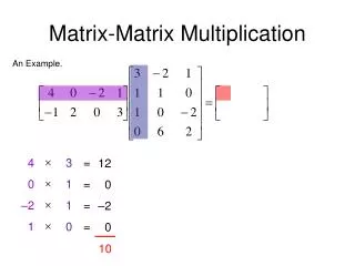
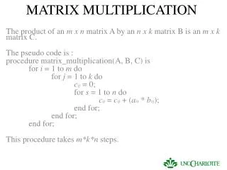
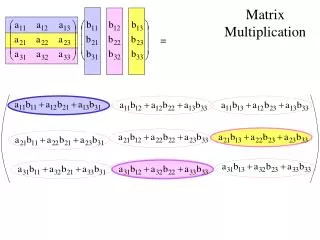
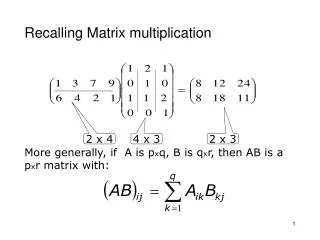
Naïve Matrix Multiply {implements C = C + A*B} for i = 1 to n for j = 1 to n for k = 1 to n C(i,j) = C(i,j) + A(i,k) * B(k,j) Algorithm has 2*n3 = O(n3) Flops and operates on 3*n2 words of memory q potentially as large as 2*n3 / 3*n2 = O(n) A(i,:) C(i,j) C(i,j) B(:,j) = + * CS267 Lecture 3
Naïve Matrix Multiply {implements C = C + A*B} for i = 1 to n {read row i of A into fast memory} for j = 1 to n {read C(i,j) into fast memory} {read column j of B into fast memory} for k = 1 to n C(i,j) = C(i,j) + A(i,k) * B(k,j) {write C(i,j) back to slow memory} A(i,:) C(i,j) C(i,j) B(:,j) = + * CS267 Lecture 3
Naïve Matrix Multiply Number of slow memory references on unblocked matrix multiply m = n3 to read each column of B n times + n2 to read each row of A once + 2n2 to read and write each element of C once = n3 + 3n2 So q = f / m = 2n3 / (n3 + 3n2) ~= 2 for large n, no improvement over matrix-vector multiply A(i,:) C(i,j) C(i,j) B(:,j) = + * CS267 Lecture 3
Matrix-multiply, optimized several ways Speed of n-by-n matrix multiply on Sun Ultra-1/170, peak = 330 MFlops CS267 Lecture 3
Naïve Matrix Multiply on RS/6000 12000 would take 1095 years T = N4.7 Size 2000 took 5 days O(N3) performance would have constant cycles/flop Performance looks like O(N4.7) CS267 Lecture 3 Slide source: Larry Carter, UCSD
Naïve Matrix Multiply on RS/6000 Page miss every iteration TLB miss every iteration Cache miss every 16 iterations Page miss every 512 iterations CS267 Lecture 3 Slide source: Larry Carter, UCSD
Blocked (Tiled) Matrix Multiply Consider A,B,C to be n-by-n matrix viewed as N-by-N matrices of b-by-b subblocks where b=n / N is called the block size for i = 1 to N for j = 1 to N {read block C(i,j) into fast memory} for k = 1 to N {read block A(i,k) into fast memory} {read block B(k,j) into fast memory} C(i,j) = C(i,j) + A(i,k) * B(k,j) {do a matrix multiply on blocks} {write block C(i,j) back to slow memory} A(i,k) C(i,j) C(i,j) = + * B(k,j) CS267 Lecture 3
Blocked (Tiled) Matrix Multiply Recall: m is amount memory traffic between slow and fast memory matrix has nxn elements, and NxN blocks each of size bxb f is number of floating point operations, 2n3 for this problem q = f / m is our measure of algorithm efficiency in the memory system So: m = N*n2 read each block of B N3 times (N3 * b2 = N3 * (n/N)2 = N*n2) + N*n2 read each block of A N3 times + 2n2 read and write each block of C once = (2N + 2) * n2 So computational intensity q = f / m = 2n3 / ((2N + 2) * n2) ~= n / N = b for large n So we can improve performance by increasing the blocksize b Can be much faster than matrix-vector multiply (q=2) CS267 Lecture 3
Using Analysis to Understand Machines The blocked algorithm has computational intensity q ~= b • The larger the block size, the more efficient our algorithm will be • Limit: All three blocks from A,B,C must fit in fast memory (cache), so we cannot make these blocks arbitrarily large • Assume your fast memory has size Mfast 3b2 <= Mfast, so q ~= b <= sqrt(Mfast/3) • To build a machine to run matrix multiply at 1/2 peak arithmetic speed of the machine, we need a fast memory of size Mfast >= 3b2 ~= 3q2 = 3(tm/tf)2 • This size is reasonable for L1 cache, but not for register sets • Note: analysis assumes it is possible to schedule the instructions perfectly CS267 Lecture 3
Limits to Optimizing Matrix Multiply • The blocked algorithm changes the order in which values are accumulated into each C[i,j] by applying associativity • Get slightly different answers from naïve code, because of roundoff - OK • The previous analysis showed that the blocked algorithm has computational intensity: q ~= b <= sqrt(Mfast/3) • There is a lower bound result that says we cannot do any better than this (using only associativity) • Theorem (Hong & Kung, 1981): Any reorganization of this algorithm (that uses only associativity) is limited to q = O(sqrt(Mfast)) • What if more levels of memory hierarchy? • Apply blocking recursively, once per level CS267 Lecture 3
Recursion: Cache Oblivious Algorithms • The tiled algorithm requires finding a good block size • Cache Oblivious Algorithms offer an alternative • Treat nxn matrix multiply set of smaller problems • Eventually, these will fit in cache • Cases for A (nxm) * B (mxp) • Case1: m>= max{n,p}: split A horizontally: • Case 2 : n>= max{m,p}: split A vertically and B horizontally • Case 3: p>= max{m,n}: split B vertically Case 2 Case 1 Case 3 CS267 Lecture 3
Experience • In practice, need to cut off recursion • Implementing a high-performance Cache-Oblivious code is not easy • Careful attention to micro-kernel and mini-kernel is needed • Using fully recursive approach with highly optimized recursive micro-kernel, Pingali et al report that they never got more than 2/3 of peak. • Issues with Cache Oblivious (recursive) approach • Recursive Micro-Kernels yield less performance than iterative ones using same scheduling techniques • Pre-fetching is needed to compete with best code: not well-understood in the context of CO codes Unpublished work, presented at LACSI 2006
Recursive Data Layouts • Blocking seems to require knowing cache sizes – portable? • A related idea is to use a recursive structure for the matrix • There are several possible recursive decompositions depending on the order of the sub-blocks • This figure shows Z-Morton Ordering (“space filling curve”) • See papers on “cache oblivious algorithms” and “recursive layouts” • Will be in next LAPACK release (Gustavson, Kagstrom, et al, SIAM Review, 2004) • Advantages: • the recursive layout works well for any cache size • Disadvantages: • The index calculations to find A[i,j] are expensive • Implementations switch to column-major for small sizes CS267 Lecture 3
Strassen’s Matrix Multiply • The traditional algorithm (with or without tiling) has O(n^3) flops • Strassen discovered an algorithm with asymptotically lower flops • O(n^2.81) • Consider a 2x2 matrix multiply, normally takes 8 multiplies, 4 adds • Strassen does it with 7 multiplies and 18 adds Let M = m11 m12 = a11 a12 b11 b12 m21 m22 = a21 a22 b21 b22 Let p1 = (a12 - a22) * (b21 + b22) p5 = a11 * (b12 - b22) p2 = (a11 + a22) * (b11 + b22) p6 = a22 * (b21 - b11) p3 = (a11 - a21) * (b11 + b12) p7 = (a21 + a22) * b11 p4 = (a11 + a12) * b22 Then m11 = p1 + p2 - p4 + p6 m12 = p4 + p5 m21 = p6 + p7 m22 = p2 - p3 + p5 - p7 Extends to nxn by divide&conquer CS267 Lecture 3
Strassen (continued) • Asymptotically faster • Several times faster for large n in practice • Cross-over depends on machine • Available in several libraries • “Tuning Strassen's Matrix Multiplication for Memory Efficiency”, M. S. Thottethodi, S. Chatterjee, and A. Lebeck, in Proceedings of Supercomputing '98 • Caveats • Needs more memory than standard algorithm • Can be less accurate because of roundoff error CS267 Lecture 3
Other Fast Matrix Multiplication Algorithms • Current world’s record is O(n 2.376... ) (Coppersmith & Winograd) • Why does Hong/Kung theorem not apply? • Possibility of O(n2+) algorithm! (Cohn, Umans, Kleinberg, 2003) • Fast methods (besides Strassen) may need unrealistically large n CS267 Lecture 3
Short Break Questions about course? Homework 1 coming soon (Friday) CS267 Lecture 3
Outline • Recap from Lecture 2 • Memory hierarchy is important to performance • Use of simple performance models to understand performance • Case Study: Matrix Multiplication • Blocking algorithms • Other tuning techniques • Alternate algorithms • Automatic Performance Tuning CS267 Lecture 3
Search Over Block Sizes • Performance models are useful for high level algorithms • Helps in developing a blocked algorithm • Models have not proven very useful for block size selection • too complicated to be useful • See work by Sid Chatterjee for detailed model • too simple to be accurate • Multiple multidimensional arrays, virtual memory, etc. • Speed depends on matrix dimensions, details of code, compiler, processor • Some systems use search over “design space” of possible implementations • Atlas – incorporated into Matlab • BeBOP – http://bebop.cs.berkeley.edu/ CS267 Lecture 3
What the Search Space Looks Like Number of columns in register block Number of rows in register block A 2-D slice of a 3-D register-tile search space. The dark blue region was pruned. (Platform: Sun Ultra-IIi, 333 MHz, 667 Mflop/s peak, Sun cc v5.0 compiler) CS267 Lecture 3
Tiling Alone Might Not Be Enough • Naïve and a “naïvely tiled” code on Itanium 2 • Searched all block sizes to find best, b=56 • Starting point for next homework CS267 Lecture 3
Optimizing in Practice • Tiling for registers • loop unrolling, use of named “register” variables • Tiling for multiple levels of cache and TLB • Exploiting fine-grained parallelism in processor • superscalar; pipelining • Complicated compiler interactions • Hard to do by hand (but you’ll try) • Automatic optimization an active research area • BeBOP: bebop.cs.berkeley.edu/ • PHiPAC: www.icsi.berkeley.edu/~bilmes/phipac in particular tr-98-035.ps.gz • ATLAS: www.netlib.org/atlas CS267 Lecture 3
Removing False Dependencies • Using local variables, reorder operations to remove false dependencies a[i] = b[i] + c; a[i+1] = b[i+1] * d; false read-after-write hazard between a[i] and b[i+1] float f1 = b[i]; float f2 = b[i+1]; a[i] = f1 + c; a[i+1] = f2 * d; • With some compilers, you can declare a and b unaliased. • Done via “restrict pointers,” compiler flag, or pragma CS267 Lecture 3
Exploit Multiple Registers • Reduce demands on memory bandwidth by pre-loading into local variables while( … ) { *res++ = filter[0]*signal[0] + filter[1]*signal[1] + filter[2]*signal[2]; signal++; } float f0 = filter[0]; float f1 = filter[1]; float f2 = filter[2]; while( … ) { *res++ = f0*signal[0] + f1*signal[1] + f2*signal[2]; signal++; } also: register float f0 = …; Example is a convolution CS267 Lecture 3
Loop Unrolling • Expose instruction-level parallelism float f0 = filter[0], f1 = filter[1], f2 = filter[2]; float s0 = signal[0], s1 = signal[1], s2 = signal[2]; *res++ = f0*s0 + f1*s1 + f2*s2; do { signal += 3; s0 = signal[0]; res[0] = f0*s1 + f1*s2 + f2*s0; s1 = signal[1]; res[1] = f0*s2 + f1*s0 + f2*s1; s2 = signal[2]; res[2] = f0*s0 + f1*s1 + f2*s2; res += 3; } while( … ); CS267 Lecture 3
Expose Independent Operations • Hide instruction latency • Use local variables to expose independent operations that can execute in parallel or in a pipelined fashion • Balance the instruction mix (what functional units are available?) f1 = f5 * f9; f2 = f6 + f10; f3 = f7 * f11; f4 = f8 + f12; CS267 Lecture 3
Copy optimization • Copy input operands or blocks • Reduce cache conflicts • Constant array offsets for fixed size blocks • Expose page-level locality Original matrix (numbers are addresses) Reorganized into 2x2 blocks 0 4 8 12 0 2 8 10 1 5 9 13 1 3 9 11 2 6 10 14 4 6 12 13 3 7 11 15 5 7 14 15 CS267 Lecture 3
ATLAS Matrix Multiply (DGEMM n = 500) Source: Jack Dongarra • ATLAS is faster than all other portable BLAS implementations and it is comparable with machine-specific libraries provided by the vendor. CS267 Lecture 3
Experiments on Search vs. Modeling • Study compares search (Atlas to optimization selection based on performance models) • Ten modern architectures • Model did well on most cases • Better on UltraSparc • Worse on Itanium • Eliminating performance gaps: think globally, search locally • -small performance gaps: local search • -large performance gaps: • refine model • Substantial gap between ATLAS CGw/S and ATLAS Unleashed on some machines CS267 Lecture 3 Source: K. Pingali. Results from IEEE ’05 paper by K Yotov, X Li, G Ren, M Garzarán, D Padua, K Pingali, P Stodghill.
Locality in Other Algorithms • The performance of any algorithm is limited by q • q = # flops / # memory refs = “Computational Intensity” • In matrix multiply, we increase q by changing computation order • Reuse data in cache (increased temporal locality) • For other algorithms and data structures, tuning still an open problem • sparse matrices (blocking, reordering, splitting) • Weekly research meetings • Bebop.cs.berkeley.edu • OSKI – tuning sequential sparse-matrix-vector multiply and related operations • trees (B-Trees are for the disk level of the hierarchy) • linked lists (some work done here) CS267 Lecture 3
Dense Linear Algebra is not All Matrix Multiply • Main dense matrix kernels are in an industry standard interface called the BLAS: Basic Linear Algebra Subroutines • www.netlib.org/blas, www.netlib.org/blas/blast--forum • Vendors, others supply optimized implementations • History • BLAS1 (1970s): • vector operations: dot product, saxpy (y=a*x+y), etc • m=2*n, f=2*n, q ~1 or less • BLAS2 (mid 1980s) • matrix-vector operations: matrix vector multiply, etc • m=n^2, f=2*n^2, q~2, less overhead • somewhat faster than BLAS1 • BLAS3 (late 1980s) • matrix-matrix operations: matrix matrix multiply, etc • m <= 3n^2, f=O(n^3), so q=f/m can possibly be as large as n, so BLAS3 is potentially much faster than BLAS2 • Good algorithms used BLAS3 when possible (LAPACK & ScaLAPACK) • Seewww.netlib.org/{lapack,scalapack} • Not all algorithms *can* use BLAS3 CS267 Lecture 3
BLAS speeds on an IBM RS6000/590 Peak speed = 266 Mflops Peak BLAS 3 BLAS 2 BLAS 1 BLAS 3 (n-by-n matrix matrix multiply) vs BLAS 2 (n-by-n matrix vector multiply) vs BLAS 1 (saxpy of n vectors) CS267 Lecture 3
Dense Linear Algebra: BLAS2 vs. BLAS3 • BLAS2 and BLAS3 have very different computational intensity, and therefore different performance Data source: Jack Dongarra CS267 Lecture 3
Other Automatic Tuning Efforts • FFTW (MIT): “Fastest Fourier Transform in the West” • Sequential (and parallel) • Many variants (real/complex, sine/cosine, multidimensional) • 1999 Wilkinson Prize • www.fftw.org • Spiral (CMU) • Digital signal processing transforms • FFT and beyond • www.spiral.net • BEBOP (UCB) • http://bebop.cs.berkeley.edu • OSKI - Sparse matrix kernels • Stencils – Structure grid kernels (with LBNL) • Interprocessor communication kernels • Bebop (UPC), Dongarra (UTK for MPI) • Class projects available CS267 Lecture 3
Summary • Performance programming on uniprocessors requires • understanding of memory system • understanding of fine-grained parallelism in processor • Simple performance models can aid in understanding • Two ratios are key to efficiency (relative to peak) • computational intensity of the algorithm: • q = f/m = # floating point operations / # slow memory references • machine balance in the memory system: • tm/tf = time for slow memory reference / time for floating point operation • Blocking (tiling) is a basic approach to increase q • Techniques apply generally, but the details (e.g., block size) are architecture dependent • Similar techniques are possible on other data structures and algorithms • Now it’s your turn: Homework 1 • Work in teams of 2 or 3 (assigned this time) CS267 Lecture 3
Reading for Today • “Parallel Computing Sourcebook” Chapters 2 & 3 • "Performance Optimization of Numerically Intensive Codes", by Stefan Goedecker and Adolfy Hoisie, SIAM 2001. • Web pages for reference: • BeBOP Homepage • ATLAS Homepage • BLAS (Basic Linear Algebra Subroutines), Reference for (unoptimized) implementations of the BLAS, with documentation. • LAPACK (Linear Algebra PACKage), a standard linear algebra library optimized to use the BLAS effectively on uniprocessors and shared memory machines (software, documentation and reports) • ScaLAPACK (Scalable LAPACK), a parallel version of LAPACK for distributed memory machines (software, documentation and reports) • Tuning Strassen's Matrix Multiplication for Memory Efficiency Mithuna S. Thottethodi, Siddhartha Chatterjee, and Alvin R. Lebeck in Proceedings of Supercomputing '98, November 1998 postscript • Recursive Array Layouts and Fast Parallel Matrix Multiplication” by Chatterjee et al. IEEE TPDS November 2002. CS267 Lecture 3
Questions You Should Be Able to Answer • What is the key to understand algorithm efficiency in our simple memory model? • What is the key to understand machine efficiency in our simple memory model? • What is tiling? • Why does block matrix multiply reduce the number of memory references? • What are the BLAS? • Why does loop unrolling improve uniprocessor performance? CS267 Lecture 3