Download
1 / 39
390 likes | 516 Views
Chapter 8 Sorting. Topics Basics Merge sort ( 合併排序 ) Quick sort Bucket sort ( 分籃排序 ) Radix sort ( 基數排序 ) Summary. Divide-and conquer ( 分化再克服 ) is a general algorithm design paradigm ( 範式 ): Divide ( 分割 ) : divide the input data S in two or more disjoint ( 分離 ) subsets S 1 , S 2 , …

E N D
Chapter 8 Sorting • Topics • Basics • Merge sort (合併排序) • Quick sort • Bucket sort (分籃排序) • Radix sort (基數排序) • Summary Merge Sort
Divide-and conquer (分化再克服) is a general algorithm design paradigm (範式): Divide (分割): dividethe input data S in two or more disjoint (分離) subsets S1, S2, … Recur (遞迴): solve (解決) the subproblems recursively (遞迴) Conquer (克服): combine (組合) the solutions (解答) for S1,S2, …, into a solution for S The base (基礎) case for the recursion are subproblems of constant (常數) size Basics Merge Sort
Merge-sort on an input sequence S with n elements consists of three steps: Divide: partition (切割) S into two sequences S1and S2 of about n/2 elements each Recur: recursively sort S1and S2 Conquer: merge (合併) S1and S2 into a unique (一個) sorted sequence Merge-Sort AlgorithmmergeSort(S, C) Inputsequence S with n elements, comparator C Outputsequence S sorted • according to C ifS.size() > 1 (S1, S2)partition(S, n/2) mergeSort(S1, C) mergeSort(S2, C) Smerge(S1, S2) Merge Sort
Merge-Sort Algorithmmerge(A, B) Inputsequences A and B withn/2 elements each Outputsorted sequence of A B S empty sequence whileA.isEmpty() B.isEmpty() ifA.first().element() < B.first().element() S.insertLast(A.remove(A.first())) else S.insertLast(B.remove(B.first())) whileA.isEmpty() S.insertLast(A.remove(A.first())) whileB.isEmpty() S.insertLast(B.remove(B.first())) return S • The conquer step of merge-sort consists of merging two sorted sequences A and B into a sorted sequence S containing (包含) the union (集合) of the elements of A and B • Merging two sorted sequences, each with n/2 elements and implemented by means of a doubly linked list, takes O(n) time Merge Sort
Merge-Sort • An execution of merge-sort is depicted (描述) by a binary tree • each node represents a recursive call of merge-sort and stores • unsorted sequence before the execution (執行) and its partition • sorted sequence at the end of the execution • the root is the initial (起始) call • the leaves (樹葉) are calls on subsequences of size 0 or 1 7 2 9 4 2 4 7 9 7 2 2 7 9 4 4 9 7 7 2 2 9 9 4 4 Merge Sort
7 2 9 4 2 4 7 9 3 8 6 1 1 3 8 6 7 2 2 7 9 4 4 9 3 8 3 8 6 1 1 6 7 7 2 2 9 9 4 4 3 3 8 8 6 6 1 1 Merge-Sort - Execution Example • Partition 7 2 9 4 3 8 6 11 2 3 4 6 7 8 9 Merge Sort
7 2 2 7 9 4 4 9 3 8 3 8 6 1 1 6 7 7 2 2 9 9 4 4 3 3 8 8 6 6 1 1 Merge-Sort - Execution Example • Recursive call, partition 7 2 9 4 3 8 6 11 2 3 4 6 7 8 9 7 2 9 4 2 4 7 9 3 8 6 1 1 3 8 6 Merge Sort
7 7 2 2 9 9 4 4 3 3 8 8 6 6 1 1 Merge-Sort - Execution Example • Recursive call, partition 7 2 9 4 3 8 6 11 2 3 4 6 7 8 9 7 2 9 4 2 4 7 9 3 8 6 1 1 3 8 6 7 2 2 7 9 4 4 9 3 8 3 8 6 1 1 6 Merge Sort
7 2 2 7 9 4 4 9 3 8 3 8 6 1 1 6 Merge-Sort - Execution Example • Recursive call, base case 7 2 9 4 3 8 6 11 2 3 4 6 7 8 9 7 2 9 4 2 4 7 9 3 8 6 1 1 3 8 6 77 2 2 9 9 4 4 3 3 8 8 6 6 1 1 Merge Sort
Merge-Sort - Execution Example • Recursive call, base case 7 2 9 4 3 8 6 11 2 3 4 6 7 8 9 7 2 9 4 2 4 7 9 3 8 6 1 1 3 8 6 7 2 2 7 9 4 4 9 3 8 3 8 6 1 1 6 77 22 9 9 4 4 3 3 8 8 6 6 1 1 Merge Sort
Merge-Sort - Execution Example • Merge 7 2 9 4 3 8 6 11 2 3 4 6 7 8 9 7 2 9 4 2 4 7 9 3 8 6 1 1 3 8 6 7 22 7 9 4 4 9 3 8 3 8 6 1 1 6 77 22 9 9 4 4 3 3 8 8 6 6 1 1 Merge Sort
Merge-Sort - Execution Example • Recursive call, …, base case, merge 7 2 9 4 3 8 6 11 2 3 4 6 7 8 9 7 2 9 4 2 4 7 9 3 8 6 1 1 3 8 6 7 22 7 9 4 4 9 3 8 3 8 6 1 1 6 77 22 9 9 4 4 3 3 8 8 6 6 1 1 Merge Sort
Merge-Sort - Execution Example • Merge 7 2 9 4 3 8 6 11 2 3 4 6 7 8 9 7 2 9 42 4 7 9 3 8 6 1 1 3 8 6 7 22 7 9 4 4 9 3 8 3 8 6 1 1 6 77 22 9 9 4 4 3 3 8 8 6 6 1 1 Merge Sort
Merge-Sort - Execution Example • Recursive call, …, merge, merge 7 2 9 4 3 8 6 11 2 3 4 6 7 8 9 7 2 9 42 4 7 9 3 8 6 1 1 3 6 8 7 22 7 9 4 4 9 3 8 3 8 6 1 1 6 77 22 9 9 4 4 33 88 66 11 Merge Sort
Merge-Sort - Execution Example • Merge 7 2 9 4 3 8 6 11 2 3 4 6 7 8 9 7 2 9 42 4 7 9 3 8 6 1 1 3 6 8 7 22 7 9 4 4 9 3 8 3 8 6 1 1 6 77 22 9 9 4 4 33 88 66 11 Merge Sort
Merge-Sort - Analysis • The height h of the merge-sort tree is O(log n) • at each recursive call we divide in half the sequence, • The overall (全部) amount (總數) or work done at the nodes of depth i is O(n) • we partition and merge 2i sequences of size n/2i • we make 2i+1 recursive calls • Thus, the total running time of merge-sort is O(n log n) Merge Sort
Quick-sort is a randomized (隨機化) sorting algorithm based on the divide-and-conquer paradigm: Divide: pick (選取) a random (隨機) element x (called pivot, 軸心) and partitionS into L elements less than x E elements equal x G elements greater than x Recur: sort L and G Conquer: join (合併) L, Eand G Quick-Sort x x L G E x Merge Sort
Quick-Sort Algorithmpartition(S,p) Inputsequence S, position p of pivot Outputsubsequences L,E, G of the elements of S less than, equal to, or greater than the pivot, resp. L,E, G empty sequences x S.remove(p) whileS.isEmpty() y S.remove(S.first()) ify<x L.insertLast(y) else if y=x E.insertLast(y) else{ y > x } G.insertLast(y) return L,E, G • We partition an input sequence as follows: • We remove, in turn, each element y from S and • We insert y into L, Eor G,depending on (依據) the result of the comparison (比較) with the pivot x • Each insertion and removal is at the beginning or at the end of a sequence, and hence takes O(1) time • Thus, the partition step of quick-sort takes O(n) time Merge Sort
Quick-Sort • An execution of quick-sort is depicted (描述) by a binary tree • Each node represents a recursive call of quick-sort and stores • Unsorted sequence before the execution and its pivot • Sorted sequence at the end of the execution • The root is the initial call • The leaves are calls on subsequences of size 0 or 1 7 4 9 6 2 2 4 6 7 9 4 2 2 4 7 9 7 9 2 2 9 9 Merge Sort
Quick-Sort - Execution Example • Pivot selection 7 2 9 4 3 7 6 11 2 3 4 6 7 8 9 7 2 9 4 2 4 7 9 3 8 6 1 1 3 8 6 9 4 4 9 3 3 8 8 2 2 9 9 4 4 Merge Sort
Quick-Sort - Execution Example • Partition, recursive call, pivot selection 7 2 9 4 3 7 6 11 2 3 4 6 7 8 9 2 4 3 1 2 4 7 9 3 8 6 1 1 3 8 6 9 4 4 9 3 3 8 8 2 2 9 9 4 4 Merge Sort
Quick-Sort - Execution Example • Partition, recursive call, base case 7 2 9 4 3 7 6 11 2 3 4 6 7 8 9 2 4 3 1 2 4 7 3 8 6 1 1 3 8 6 11 9 4 4 9 3 3 8 8 9 9 4 4 Merge Sort
Quick-Sort - Execution Example • Recursive call, …, base case, join 7 2 9 4 3 7 6 11 2 3 4 6 7 8 9 2 4 3 1 1 2 3 4 3 8 6 1 1 3 8 6 11 4 334 3 3 8 8 9 9 44 Merge Sort
Quick-Sort - Execution Example • Recursive call, pivot selection 7 2 9 4 3 7 6 11 2 3 4 6 7 8 9 2 4 3 1 1 2 3 4 7 9 7 1 1 3 8 6 11 4 334 8 8 9 9 9 9 44 Merge Sort
Quick-Sort - Execution Example • Partition, …, recursive call, base case 7 2 9 4 3 7 6 11 2 3 4 6 7 8 9 2 4 3 1 1 2 3 4 7 9 7 1 1 3 8 6 11 4 334 8 8 99 9 9 44 Merge Sort
Quick-Sort - Execution Example • Join, join 7 2 9 4 3 7 6 1 1 2 3 4 67 7 9 2 4 3 1 1 2 3 4 7 9 7 1779 11 4 334 8 8 99 9 9 44 Merge Sort
Quick-Sort - Analysis • The worst case for quick-sort occurs when the pivot is the unique minimum or maximum element • One of L and G has size n - 1 and the other has size 0 • The running time is proportional to the sum n+ (n- 1) + … + 2 + 1 • Thus, the worst-case running time of quick-sort is O(n2) … Merge Sort
Consider a recursive call of quick-sort on a sequence of size s Good call: the sizes of L and G are each less than 3s/4 Bad call: one of L and G has size greater than 3s/4 A call is good with probability 1/2 1/2 of the possible pivots cause good calls: 1 2 3 4 5 6 7 8 9 10 11 12 13 14 15 16 Quick-Sort - Analysis 7 2 9 4 3 7 6 1 9 7 2 9 4 3 7 6 1 1 7 2 9 4 3 7 6 2 4 3 1 7 9 7 1 1 Good call Bad call Bad pivots Good pivots Bad pivots Merge Sort
Probabilistic Fact: The expected number of coin tosses required in order to get k heads is 2k For a node of depth i, we expect i/2 ancestors are good calls The size of the input sequence for the current call is at most (3/4)i/2n Quick-Sort - Analysis • Therefore, we have • For a node of depth 2log4/3n, the expected input size is one • The expected height of the quick-sort tree is O(log n) • The amount (總數) or work done at the nodes of the same depth is O(n) • Thus, the expected running time of quick-sort is O(n log n) Merge Sort
Quick-Sort – In-Place Sort • Quick-sort can be implemented to run in-place • In the partition step, we use replace operations to rearrange the elements of the input sequence such that • the elements less than the pivot have rank less than h • the elements equal to the pivot have rank between h and k • the elements greater than the pivot have rank greater than k • The recursive calls consider • elements with rank less than h • elements with rank greater than k AlgorithminPlaceQuickSort(S,l,r) Inputsequence S, ranks l and r Output sequence S with the elements of rank between l and rrearranged in increasing order ifl r return i a random integer between l and r x S.elemAtRank(i) (h,k) inPlacePartition(x) inPlaceQuickSort(S,l,h - 1) inPlaceQuickSort(S,k + 1,r) Merge Sort
Quick-Sort – In-Place Sort • Perform the partition using two indices to split S into L and E U G (a similar method can split E U G into E and G). • Repeat until j and k cross: • Scan j to the right until finding an element > x. • Scan k to the left until finding an element < x. • Swap elements at indices j and k j k (pivot = 6) 3 2 5 1 0 7 3 5 9 2 7 9 8 9 7 6 9 j k 3 2 5 1 0 7 3 5 9 2 7 9 8 9 7 6 9 Merge Sort
Quick-Sort - Java Implementation public static void quickSort (Object[] S, Comparator c) { if (S.length < 2) return; // the array is already sorted in this case quickSortStep(S, c, 0, S.length-1); // recursive sort method } private static void quickSortStep (Object[] S, Comparator c, int leftBound, int rightBound ) { if (leftBound >= rightBound) return; // the indices have crossed Object temp; // temp object used for swapping Object pivot = S[rightBound]; int leftIndex = leftBound; // will scan rightward int rightIndex = rightBound-1; // will scan leftward while (leftIndex <= rightIndex) { // scan right until larger than the pivot while ( (leftIndex <= rightIndex) && (c.compare(S[leftIndex], pivot)<=0) ) leftIndex++; // scan leftward to find an element smaller than the pivot while ( (rightIndex >= leftIndex) && (c.compare(S[rightIndex], pivot)>=0)) rightIndex--; if (leftIndex < rightIndex) { // both elements were found temp = S[rightIndex]; S[rightIndex] = S[leftIndex]; // swap these elements S[leftIndex] = temp; } } // the loop continues until the indices cross temp = S[rightBound]; // swap pivot with the element at leftIndex S[rightBound] = S[leftIndex]; S[leftIndex] = temp; // the pivot is now at leftIndex, so recurse quickSortStep(S, c, leftBound, leftIndex-1); quickSortStep(S, c, leftIndex+1, rightBound); } only works for distinct elements Merge Sort
Let be S be a sequence of n (key, element) entries with keys in the range [0, N- 1] Bucket-sort uses the keys as indices into an auxiliary array B of sequences (N buckets) Phase 1: Empty sequence S by moving each entry (k, o) into its bucket B[k] Phase 2: For i = 0, …,N -1, move the entries of bucket B[i] to the end of sequence S Analysis: Phase 1 takes O(n) time Phase 2 takes O(n+ N) time Bucket-sort takes O(n+ N) time Bucket-Sort AlgorithmbucketSort(S,N) Inputsequence S of (key, element) items with keys in the range [0, N- 1]Outputsequence S sorted by increasing keys B array of N empty sequences whileS.isEmpty() f S.first() (k, o) S.remove(f) B[k].insertLast((k, o)) for i 0 toN -1 whileB[i].isEmpty() f B[i].first() (k, o) B[i].remove(f) S.insertLast((k, o)) Merge Sort
7, d 1, c 3, a 7, g 3, b 7, e 1, c 3, a 3, b 7, d 7, g 7, e B 0 1 2 3 4 5 6 7 8 9 1, c 3, a 3, b 7, d 7, g 7, e Bucket-Sort - Example • Key range [0, 9] Phase 1 Phase 2 Merge Sort
Key-type Property The keys are used as indices into an array and cannot be arbitrary objects No external (外在) comparator (比較子) Stable Sort Property The relative order of any two items with the same key is preservedafter the execution of the algorithm Extensions Integer keys in the range [a, b] Put entry (k, o) into bucketB[k - a] String keys from a set D of possible strings, where D has constant size (e.g., names of the 50 U.S. states) Sort D and compute the rank r(k)of each string k of D in the sorted sequence Put entry (k, o) into bucket B[r(k)] Bucket-Sort - Properties and Extensions Merge Sort
Radix-sort is a specialization (特例) of lexicographic-sort that uses bucket-sort as the stable sorting algorithm in each dimension Radix-sort is applicable to tuples where the keys in each dimension i are integers in the range [0, N- 1] Radix-sort runs in time O(d( n+ N)) Radix-Sort AlgorithmradixSort(S, N) Inputsequence S of d-tuples such that (0, …, 0) (x1, …, xd) and (x1, …, xd) (N- 1, …, N- 1) for each tuple (x1, …, xd) in SOutputsequence S sorted in lexicographic order for i ddownto 1 bucketSort(S, N) Merge Sort
Radix-Sort – Example • Consider a sequence of nb-bit integers x=xb- 1 … x1x0 • We represent each element as a b-tuple of integers in the range [0, 1] and apply radix-sort with N= 2 • This application of the radix-sort algorithm runs in O(bn) time • For example, we can sort a sequence of 32-bit integers in linear time AlgorithmbinaryRadixSort(S) Inputsequence S of b-bit integers Outputsequence S sorted replace each element x of S with the item (0, x) for i 0 tob - 1 replace the key k of each item (k, x) of S with bit xi of x bucketSort(S, 2) Merge Sort
1001 1001 1001 0001 0010 0010 0010 1101 0001 1110 1101 1001 0001 0010 1001 1101 0001 0010 1101 1101 1110 1110 1110 1110 0001 Radix-Sort - Example • Sorting a sequence of 4-bit integers Merge Sort
Summary Merge Sort