Download
1 / 77
770 likes | 978 Views
Statistics in WR: Lecture 1. Key Themes Knowledge discovery in hydrology Introduction to probability and statistics Definition of random variables Reading: Helsel and Hirsch, Chapter 1. By deduction from existing knowledge By experiment in a laboratory

E N D
Statistics in WR: Lecture 1 • Key Themes • Knowledge discovery in hydrology • Introduction to probability and statistics • Definition of random variables • Reading: Helsel and Hirsch, Chapter 1
By deduction from existing knowledge By experiment in a laboratory By observation of the natural environment How is new knowledge discovered? After completing the Handbook of Hydrology in 1993, I asked myself the question: how is new knowledge discovered in hydrology? I concluded:
Deduction is the classical path of mathematical physics Given a set of axioms Then by a logical process Derive a new principle or equation In hydrology, the St Venant equations for open channel flow and Richard’s equation for unsaturated flow in soils were derived in this way. Deduction – Isaac Newton Three laws of motion and law of gravitation http://en.wikipedia.org/wiki/Isaac_Newton (1687)
Experiment is the classical path of laboratory science – a simplified view of the natural world is replicated under controlled conditions In hydrology, Darcy’s law for flow in a porous medium was found this way. Experiment – Louis Pasteur Pasteur showed that microorganisms cause disease & discovered vaccination Foundations of scientific medicine http://en.wikipedia.org/wiki/Louis_Pasteur
Observation – direct viewing and characterization of patterns and phenomena in the natural environment In hydrology, Horton discovered stream scaling laws by interpretation of stream maps Observation – Charles Darwin Published Nov 24, 1859 Most accessible book of great scientific imagination ever written
Is there a relation between flow and water quality? Total Nitrogen in water
CE 397 Statistics in Water Resources, Lecture 2, 2009 David R. Maidment Dept of Civil Engineering University of Texas at Austin
Key Themes • Statistics • Parametric and non-parametric approach • Data Visualization • Distribution of data and the distribution of statistics of those data • Reading: Helsel and Hirsch p. 17-51 (Sections 2.1 to 2.3 • Slides from Helsel and Hirsch (2002) “Techniques of water resources investigations of the USGS, Book 4, Chapter A3.
Characteristics of Water Resources Data • Lower bound of zero • Presence of “outliers” • Positive skewness • Non-normal distribution of data • Data measured with thresholds (e.g. detection limits) • Seasonal and diurnal patterns • Autocorrelation – consecutive measurements are not independent • Dependence on other uncontrolled variables e.g. chemical concentration is related to discharge
Normal Distribution From Helsel and Hirsch (2002)
Lognormal Distribution From Helsel and Hirsch (2002)
Method of Moments From Helsel and Hirsch (2002)
Statistical measures • Location (Central Tendency) • Mean • Median • Geometric mean • Spread (Dispersion) • Variance • Standard deviation • Interquartile range • Skewness (Symmetry) • Coefficient of skewness • Kurtosis (Flatness) • Coefficient of kurtosis
Histogram From Helsel and Hirsch (2002) Annual Streamflow for the Licking River at Catawba, Kentucky 03253500
Quantile Plot From Helsel and Hirsch (2002)
Plotting positions i = rank of the data with i = 1 is the lowest n = number of data p = cumulative probability or “quantile” of the data value (its percentile value)
Normal Distribution Quantile Plot From Helsel and Hirsch (2002)
Probability Plot with Normal Quantiles(Z values) q z From Helsel and Hirsch (2002)
Annual Flows From HydroExcel Annual Flows produced using Pivot Tables in Excel
CE 397 Statistics in Water Resources, Lecture 3, 2009 David R. Maidment Dept of Civil Engineering University of Texas at Austin
Key Themes • Using HydroExcel for accessing water resources data using web services • Descriptive statistics and histograms using Excel Analysis Toolpak • Reading: Chapter 11 of Applied Hydrology by Chow, Maidment and Mays
CE 397 Statistics in Water Resources, Lecture 4, 2009 David R. Maidment Dept of Civil Engineering University of Texas at Austin
Key Themes • Frequency and probability functions • Fitting methods • Typical distributions • Reading: Chapter 4 of Helsel and Hirsh pp. 97-116 on Hypothesis tests
CE 397 Statistics in Water Resources, Lecture 5, 2009 David R. Maidment Dept of Civil Engineering University of Texas at Austin
Key Themes • Using Excel to fit frequency and probability distributions • Chi Square test and probability plotting • Beginning hypothesis testing • Reading: Chapter 3 of Helsel and Hirsh pp. 65-97 on Describing Uncertainty • Slides from Helsel and Hirsch Chap. 4
Statistics in Water Resources, Lecture 6 • Key theme • T-distribution for distributions where standard deviation is unknown • Hypothesis testing • Comparing two sets of data to see if they are different • Reading: Helsel and Hirsch, Chapter 6 Matched Pair Tests
Chi-Square Distribution http://en.wikipedia.org/wiki/Chi-square_distribution
t-, z and ChiSquare Source: http://en.wikipedia.org/wiki/Student's_t-distribution
Normal and t-distributions Normal t-dist for ν = 1 t-dist for ν = 3 t-dist for ν = 2 t-dist for ν = 5 t-dist for ν = 10 t-dist for ν = 30
Standard Normal and Student - t • Standard Normal z • X1, … , Xn are independently distributed (μ,σ), and • then is normally distributed with mean 0 and std dev 1 • Student’s t-distribution • Applies to the case where the true standard deviation σ is unknown and is replaced by its sample estimate Sn
p-value is the probability of obtaining the value of the test-statistic if the null hypothesis (Ho) is true If p-value is very small (<0.05 or 0.025) then reject Ho If p-value is larger than α then do not reject Ho
Statistics in WR: Lecture 7 • Key Themes • Statistics for populations and samples • Suspended sediment sampling • Testing for differences in means and variances • Reading: Helsel and Hirsch Chapter 8 Correlation
Estimators of the Variance Maximum Likelihood Estimate for Population variance Unbiased estimate from a sample http://en.wikipedia.org/wiki/Variance
Bias in the Variance Common sense would suggest to apply the population formula to the sample as well. The reason that it is biased is that the sample mean is generally somewhat closer to the observations in the sample than the population mean is to these observations. This is so because the sample mean is by definition in the middle of the sample, while the population mean may even lie outside the sample. So the deviations from the sample mean will often be smaller than the deviations from the population mean, and so, if the same formula is applied to both, then this variance estimate will on average be somewhat smaller in the sample than in the population.
Suspended Sediment Sampling http://pubs.usgs.gov/sir/2005/5077/
Statistics in WR: Lecture 8 • Key Themes • Replication in Monte Carlo experiments • Testing paired differences and analysis of variance • Correlation • Reading: Helsel and Hirsch Chapter 9 Simple Regression
Patterns of data that all have correlation between x and y of 0.7
Monotonic nonlinear correlation Linear correlation Non-monotonic correlation