Download
1 / 24
240 likes | 437 Views
CLIC Drive Beam Beam Position Monitors International Workshop on Linear Colliders 2010 Geneva Steve Smith SLAC / CERN 20.10.2010. CLIC Accelerator Complex. RF (klystron) power goes into drive beam efficiently: high current, long pulse, low energy, 500 MHz

E N D
CLIC Drive Beam Beam Position MonitorsInternational Workshop on Linear Colliders 2010GenevaSteve SmithSLAC / CERN20.10.2010
CLIC Accelerator Complex • RF (klystron) power goes into drive beam efficiently: • high current, long pulse, low energy, 500 MHz • Compress drive beam to high current, high frequency • Transfer energy to main beam
CLIC Acceleration Scheme • Drive beam linac: • high current (4 Amp), • long pulse (140 µs), • low energy (2.38 GeV) • modest RF frequency (500 MHz) • Compress train length in Delay Loop, Combiner Rings • multiply bunch frequency by 24 • From 500 MHz to 12 GHz • Split each drive beam into 24 sub-trains • 240 ns each • Decelerate drive beam / accelerate main beam • 24 decelerators segments per main beam linac • 800 m each • 12 GHz • 100 Amp • 90% energy extraction
Beam Position Monitors • Main Beam • Quantity ~7500 • Including: • 4196 Main beam linac • 50 nm resolution • 1200 in Damping & Pre-Damping Ring • Drive Beam • Quantity ~45000 • 660 in drive beam linacs • 2792 in transfer lines and turnarounds • 41000 in drive beam decelerators • !
CLIC Drive Beam Decelerator BPMs • Requirements • Transverse resolution < 2 microns • Temporal resolution < 10 ns • Bandwidth > 20 MHz • Accuracy < 20 microns • Wakefields must be low • Consider Pickups: • Resonant cavities • Striplines • Buttons
Drive Beam Decelerator BPM Challenges • Bunch frequency in beam: 12 GHz • Lowest frequency intentionally in beam spectrum • It is above waveguide propagation cutoff • TE11 ~ 7.6 GHz for 23 mm aperture • There may be non-local beam signals above waveguide cutoff. • 130 MW @ 12 GHz Intentionally propagating in nearby Power Extraction Structures (PETS) • Consider resonant BPM operating at 12 GHz: • Plenty of signal • But sensitive to waveguide mode propagating in beampipe • Would need to kill tails of 12 GHz modes very cleanly
Operating Frequency • Study operation at sub-harmonic of bunch spacing • Example: FBPM = 2 GHz • Signal is sufficient • Especially at harmonics of drive beam linac RF • Could use • buttons • compact striplines • But there exist confounding signals • Baseband • Bandwidth ~ 4 - 40 MHz • traditional • resolution is adequate • Check temporal resolution • Requires striplines to get adequate S/N at low frequencies (< 10 MHz)
Generic Stripline BPM • Algorithm: • Measure amplitudes on 4 strips • Resolution: • Small difference in big numbers • Calibration is crucial! Given: R = 11.5 mm and sy < 2 mm Requires sV/Vpeak = 1/6000 12 effective bits
Decelerator Stripline BPM striplines Diameter: 23 mm Stripline length: 25 mm Width: 12.5% of circumference (per strip) Impedance: 50 Ohm Quad
Signal Processing Scheme • Lowpass filter to ~ 20 MHz • Digitize with fast ADC • 160 Msample/sec • 16 bits, 12 effective • Assume noise figure ≤10 dB Including Cable & filter losses amplifier noise figure ADC noise • For nominal single bunch charge 8.3 nC • Single bunch resolution y < 1 mm
Single Bunch and Train Transient Repsonse • What about the turn-on / turn-off transients of the nominal fill pattern? • Provides good position measurement for head/tail of train • Example: NLCTA • ~100 ns X-band pulse • BPM measured head & tail position with 5 - 50 MHz bandwidth • CLIC Decelerator BPM: • Single Bunch Full Train • Q=8.3 nC I = 100 Amp • y ~ 2 mm y < 1 mm (train of at least 4 bunches)
Temporal Response within Train • Transverse oscillation at 10 MHz with 2 micron amplitude • Stripline difference signal Up-Down: • S/Nthermal huge but ADC noise limit: ~ 2 m/Nsample
Where do Position Signals Originate? • Convolute pickup source term • for up/down electrodes • to first order in position y • With stripline response function • where Z is impedance and • l is the length of strip • At low frequency < c/2L ~ 6GHz • Looks like Up-Down Difference: • In middle of train we measure position via Q*d/dt(y) signal • Difference signal starts/ends in phase w/ position • but is in quadrature away from initial/final transient • In order to reconstruct position vs. time along train • must measure response function with single/few bunches
Summary of Performance • Single Bunch • For nominal bunch charge Q=8.3 nC • y ~ 2 mm • Train-end transients • For current I = 100 Amp y < 1 mm (train of at least 4 bunches) • For full 240 ns train length • current I > 1 Amp • y < 1 mm • Within train • For nominal beam current ~ 100 A sy ~ 2 mm for t > 20 ns
Calibration Calibrate Y Calibrate X • Transmit calibration from one strip • Measure ratio of couplings on adjacent striplines • Repeat on other axis • Gain ratio BPM Offset • Repeat between accelerator pulses • Transparent to operations • Very successful at LCLS
Finite-Element Calculation • Characterize beam-BPM interaction • GDFIDL • Thanks to Igor Syratchev • Geometry from BPM design files • Goals: • Check calculations where we have analytic approximations • Signal • Wakes • Look for • trapped modes • Mode purity Port Signal Transverse Wake
Transverse Wake • Find unpleasant trapped mode near 12 GHz (!) • Add damping material around shorted end of stripline • Results: • Mode damped • Response essentially unchanged at signal frequency Transverse Wake
Damped Stripline BPM Damping Material • Few mm thick ring of SiC • Transverse mode fixed • Signal not affected materially • Slight frequency shift Wake __ Damped __ Undamped Signal Transverse Impedance Signal Spectrum
Comparison to GDFIDL • Compare to analytical calculation of “perfect stripline” • Find resonant frequencies don’t match • GDFIDL ~ 2.3 GHz • Analytic model is 3 GHz • Is this due to dielectric loading due to absorber material? • Amplitudes in 100 MHz around 2 GHZ differ by only ~5% (!) • Energy integrated over 1 bunch: • 0.16 fJ GDFIDL • 0.15 fJ Mathcad • Must be some luck here • filter functions are different • resonance frequencies don’t match • Effects of dielectric loading partially cancels • Lowers frequency of peak response raises signal below peak • Reduces Z decreases signal
Sensitivity • Ratio of Dipole to Monopole • D/S ratio • GDFIDL calculation • Signal in 100 MHz bandwidth around 2 GHz • Monopole 1.75 mV/pC • Dipole 0.25 mV/pC • Ratio 0.147/mm • Theory • y = R/2*D/S • Ratio of dipole/monople = 2/R = 0.148/mm for R =13.5 mm • (R of center of stripline, it’s not clear exactly which R to use here) • Excellent agreement for transverse scale
Multibunch Transverse Wake • Calculate transverse wakefield: • GDFIDL shows quasi-DC Component: 30.6 mV/pC/mm/BPM • Calculate 27 mV/pC/mm/BPM for ideal stripline • Excellent agreement • Components at 12 GHz, 24 GHz, 36 GHz: • Comparable to features of PETS • Compare with GDFIDL:
Longitudinal Wakefrom GDFIDL Multibunch: • No coherent buildup • Peak voltage unchanged • Multiply by bunch charge in pC to get wake • 8.3 nC/bunch Single Bunch
Summary of Comparison to GDFIDL • GDFIDL and analytic calculation agree very well on characteristics • Signals at ports: • Monopole • Dipole • Transverse Wake • Disagree on response null at signal port • May need lowpass filter to reduce 12 GHz before cables • Signal Characteristics Good • Longitudinal & transverse wakes Good
Summary • A conventional stripline BPM should satisfy requirements • Processing basband (0 – 40 MHz) stripline signals • Signals are local • Calculation agrees with simulation: • Wakefields • Trapped modes • Can achieve required resolution • Calibrate carefully • Online • transparently • Should have accuracy of typical BPM of this diameter • Pay attention to source of BPM signal • Need to unfold position signal y(t) • Occasionally measure response functions • with single/few bunch beam