Download
1 / 46
470 likes | 587 Views
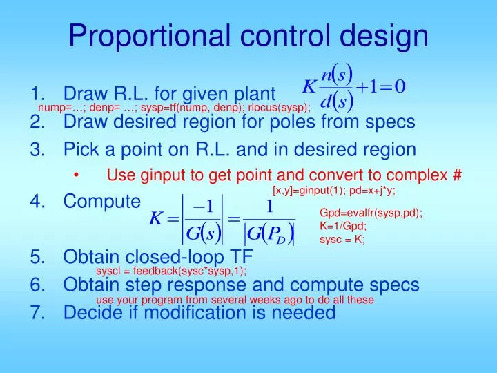
Proportional control design. Draw R.L. for given plant Draw desired region for poles from specs Pick a point on R.L. and in desired region Use ginput to get point and convert to complex # Compute Obtain closed-loop TF Obtain step response and compute specs Decide if modification is needed.

E N D
Proportional control design • Draw R.L. for given plant • Draw desired region for poles from specs • Pick a point on R.L. and in desired region • Use ginput to get point and convert to complex # • Compute • Obtain closed-loop TF • Obtain step response and compute specs • Decide if modification is needed nump=…; denp= …; sysp=tf(nump, denp); rlocus(sysp); [x,y]=ginput(1); pd=x+j*y; Gpd=evalfr(sysp,pd); K=1/Gpd; sysc = K; syscl = feedback(sysc*sysp,1); use your program from several weeks ago to do all these
PD controller design Design steps: • From specs, draw desired region for pole.Pick from region, not on RL • Compute • Select • Select: [x,y]=ginput(1); pd=x+j*y; Gpd=evalfr(sysp,pd) phi=pi - angle(Gpd) z=abs(real(pd))+abs(imag(pd)/tan(phi)); Kd=1/abs(pd+z)/abs(Gpd); Kp=z*Kd;
Approximation to PD • Same usefulness as PD • Lead Control: • Draw R.L. for G • From specs draw region for desired c.l. poles • Select pd from region • LetPick –z somewhere below pd on –Re axisLetSelect [x,y]=ginput(1); pd=x+j*y; Gpd=evalfr(sysp,pd) phi=pi - angle(Gpd) [x,y]=ginput(1); z=abs(x); phi1=angle(pd+z); phi2=phi1-phi; p=abs(real(pd))+abs(imag(pd)/tan(phi2)); K=abs((pd+p)/(pd+z)/Gpd); sysc=tf(K*[1 z],[1 p]); Hold on; rlocus(sysc*sysp);
Alternative Lead Control • Draw R.L. for G • From specs draw region for desired c.l. poles • Select pd from region • Let • Select phipd=angle(pd); phi1=(phipd+phi)/2; phi2=phi1-phi;
Lag Design steps • Draw R.L. for G(s). • From specs, draw desired pole region • Select pd on R.L. & in region • Get • With that K, compute error constant(Kpa, Kva, Kaa) from KG(s) • From specs, compute Kpd, Kvd, Kad P sysol = sysc*sysp; [nol, dol]=tfdata(sysol,'v'); dn0=dol(dol~=0); Kact=nol(end)/dn0(end); Kdes = 1/ess;
If Kact > Kdes , doneelse: pick • Re-compute • Closed-loop simulation & tuning as necessary z=-real(pd)/…; p=z*Kact/Kdes/(1+…); 0.05 or 0.1 K from 8 should be ~1, so 8 is normally skipped.
PI Design steps First PI design (a special Lag design): • Draw R.L. for G(s) • From specs, draw desired region • Pick pd on R.L. & in region • i. Chooseii. Choose • Simulate & tune
Alternative PI design • Since PI = PD/s, • Can first multiply system by 1/s • Then design using PD • The overall controller is the controller you designed divided by s
Overall controller design • Draw R.L. for G(s), hold graph • Draw desired region for closed-loop poles based on desired specs • If R.L. goes through region, pick pd on R.L. and in region. Go to step 7. R(s) E(s) C(s) U(s) Gp(s) Y(s)
Pick pd in region (near corner but inside region for safety margin) • Compute angle deficiency: • a. PD control, choose zpd such that then
b. Lead control: choose zlead, plead such thatYou can select zlead & compute plead. Or you can use the “bisection” method to compute z and p. Then If f < 60~70 deg, a single stage of PD or lead will work. If f > 80~90 deg, use a two-lead or PD-lead controller.
Compute overall gain: • If there is no steady-state error requirement, go to 14. • With K from 7, evaluate error constant that you already have:
The 0, 1, 2 should match p, v, a This is for lag control. For PI:
Compute desired error const. from specs: • For PI : set K*a = K*d & solve for zpiFor lag : pick zlag & let
Re-compute K (this step may be unnecessary) • Get closed-loop T.F. Do step response analysis. • If not satisfactory, go back to 3 and redesign.
Control System Implementation R(s) E(s) C(s) U(s) Gp(s) Y(s) disturbance input Reference Command output error Controller control Actuator Plant + plant input _ Sensor noise
PC-in-the-loop Control disturbance input Reference Command PC I/O I/O output D/A Power Amp Actuator Plant Signal conditioner and amplifier A/D Sensor All control algorithms implemented in PC (could be Matlab Real-Time) Needs data acquisition system, including A/D and D/A Needs power amplifier
m-Controller based control disturbance input Reference Command m-Controller I/O I/O output Power Amp Actuator Plant Signal conditioner and amplifier Sensor Very similar architecture to PC-in-the-loop control All control algorithms implemented in m-controller m-controller has its own A/D and D/A, but make sure resolution is OK Still needs power amplifier, because m-controller outputs weak signal
Power electronic based control disturbance input Reference Command Difference amplifier output Op Amp circuit Actuator Plant Sensor Analog operation, fastest Inexpensive All algorithms in circuit hardware Op Amp circuits for various controllers are given in book No sampling and aliasing issues
Difference Amplifier Example circuit: R2 R1 r + − e y R3 R4
Op-amp controller circuit: • Proportional: R2 R4 R1 R3 − + e − + u
Integral: C1 R4 R1 R3 − + e − + u
Derivative control: R4 R2 C1 R3 − + e − + u
PD controller: R4 R2 C1 R3 − + e − + u R1
PI controller: C1 R4 R2 R1 R3 − + e − + u
PID controller: C2 R4 R2 R1 R3 − + e − + u C1
Lead or lag controller: C2 R4 R2 R1 R3 − + e − + u C1
If R1C1 > R2C2then z < pThis is lead controller If R1C1 < R2C2then z > pThis is lag controller
Lead-lag controller: C2 R2 R4 R6 R1 C1 R5 − + e − + u R3
Example: Want: Solution: Draw R.L. C(s) Gp(s)
Clearly, R.L. pass through desired region. Pick (right on boundary) Choose
Step response: ess = 0 No MP (no overshoot) fast rise to 0.85, then very sluggish to 1 Tune 1: KP↑ to 2.5 KP
None unique solution • Design is a creative process guided by science
C(s) G(s) Example: Want:
Sol: G(s) is type 1Since we want finite ess to unit acc, we need the compensated system to be type 2C(s) needs to have in it
Draw R.L., it passes through the desired region. Pick pd on R.L. & in Region pick pd = – 180 + j160 Now choose z to meet Ka:
Pick z = 0.03 Do step resp. of closed-loop: Is it good enough?