Download

1 / 18
180 likes | 272 Views
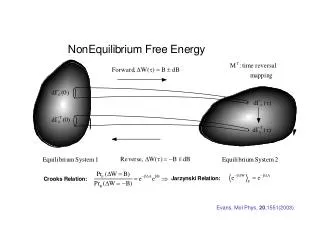
Evans, Mol Phys, 20 ,1551(2003). Jarzynski Equality proof:. systems are deterministic and canonical. Crooks proof:. Jarzynski and NPI. Take the Jarzynski work and decompose into into its reversible and irreversible parts.

E N D
Jarzynski Equality proof: systems are deterministic and canonical Crooks proof:
Jarzynski and NPI. Take the Jarzynski work and decompose into into its reversible and irreversible parts. Then we use the NonEquilibrium Partition Identity to obtain the Jarzynski work Relation:
Proof of generalized Jarzynski Equality. For any ensemble we define a generalized “work” function as: We observe that the Jacobian gives the volume ratio:
We now compute the expectation value of the generalized work. If the ensembles are canonical and if the systems are in contact with heat reservoirs at the same temperature QED
NEFER for thermal processes Assume equations of motion Then from the equation for the generalized “work”:
Generalized “power” Classical thermodynamics gives
• small system • short trajectory • small external forces Strategy of experimental demonstration of the FTs • single colloidal particle • position & velocity measured precisely • impose & measure small forces . . . measure energies, to a fraction of , along paths
Optical Trap Schematic r Photons impart momentum to the particle, directing it towards the most intense part of the beam. k < 0.1 pN/m, 1.0 x 10⁻⁵ pN/Å
Optical Tweezers Lab quadrant photodiode position detector sensitive to 15 nm, means that we can resolve forces down to 0.001 pN or energy fluctuations of 0.02 pN nm (cf. kBT=4.1 pN nm)
vopt= 1.25mm/sec 0 t=0 time For the drag experiment... velocity As DA=0, and FT and Crooks are “equivalent” Wt > 0, work is required to translate the particle-filled trap Wt < 0, heat fluctuations provide useful work “entropy-consuming” trajectory Wang, Sevick, Mittag, Searles & Evans, “Experimental Demonstration of Violations of the Second Law of Thermodynamics”Phys. Rev. Lett. (2002)
First demonstration of the (integrated) FT FT shows that entropy-consuming trajectories are observable out to 2-3 seconds in this experiment Wang, Sevick, Mittag, Searles & Evans, Phys. Rev. Lett.89, 050601 (2002)
Histogram of Wt for Capture predictions from Langevin dynamics k0 = 1.22 pN/mm k1 = (2.90, 2.70) pN/mm Carberry, Reid, Wang, Sevick, Searles & Evans, Phys. Rev. Lett. (2004)
NPI ITFT The LHS and RHS of the Integrated Transient Fluctuation Theorem (ITFT) versus time, t. Both sets of data were evaluated from 3300 experimental trajectories of a colloidal particle, sampled over a millisecond time interval. We also show a test of the NonEquilibrium Partition Identity. (Carberry et al, PRL, 92, 140601(2004))
Summary Exptl Tests of Steady State Fluctuation Theorem •Colloid particle 6.3 µm in diameter. • The optical trapping constant, k, was determined by applying the equipartition theorem: k = kBT/<r2>. •The trapping constant was determined to be k = 0.12 pN/µm and the relaxation time of the stationary system was t =0.48 s. • A single long trajectory was generated by continuously translating the microscope stage in a circular path. • The radius of the circular motion was 7.3 µm and the frequency of the circular motion was 4 mHz. • The long trajectory was evenly divided into 75 second long, non-overlapping time intervals, then each interval (670 in number) was treated as an independent steady-state trajectory from which we constructed the steady-state dissipation functions.