Download
1 / 15
150 likes | 281 Views
1.3 Density Curves and Normal Distributions. What is a density curve?. Idea of density. Density curve describes an overall pattern. Area under the curve should give a probability- hence, total area under a density curve is always 1. We would like to model real life data by a density curve.

E N D
Idea of density Density curve describes an overall pattern. Area under the curve should give a probability- hence, total area under a density curve is always 1. We would like to model real life data by a density curve.
Population vs. Sample Whenever we use a histogram to approximate a density curve, we must be careful to distinguish between the mean of the sample vs. the mean of the population. Likewise for standard deviation. We use x for the mean of the sample and the Greek letter μ (mu) for the mean of the population. Note that while we may never know μ, it does exist. We use s for standard deviation of sample and σ (sigma) for the population standard deviation.
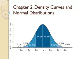
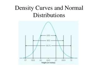
Normal Distributions When a density distribution is symmetric, we say this is a normal distribution. Normal distributions can have different shapes.
It turns out that a normal curve is completely determined by the mean and standard deviation. Mean is at the maximum point. 1 Standard deviation is where the curve changes “concavity.” 68%-95%-99.7% rule
The general formula (which you will not need to know or use for this class) for a normal distribution is given by • Notice that the mean and standard deviation completely characterize a normal curve.
Keeping our discussion of the normal curve in mind, we consider a special normal curve (and hence special continuous distribution) by letting μ=0 and σ=1. This is the standard normal variable, usually denoted z. • Table A in the back of the book gives “z-scores” for a standard normal distribution. • We will see that any continuous distribution may be “scaled” to standard by shifting the numbers so that their mean is 0 and declaring that the standard deviation constitutes a single unit • First an example.
For the standard normal random variable, find • P(0<z<1.23) • P(-1.04<z) • P(-.65<z<1.82) • P(z>1.25 or z<-1.25) • We can also answer the following question: P(z>?)=.22
Any normal distribution can be “scaled” and thought of as a standard normal distribution. To see how this is done, consider a normal variable x with mean μ and standard deviation σ. We define the standard score or z-score to be
This does exactly what we want. For example, when x=μ, we get a value of 0. • Let μ=50 and σ=5. If x=60, we can see that x is 2 standard deviations above the mean. This is also seen by plugging in the values into the z-score formula. Hence, the z-score also tells us how many standard deviations away from the mean a particular value is.
Examples • Consider a normal random variable with mean 40 and standard deviation 15. What percentage of values are • Larger than 60? • Less than 45? • Between 33 and 43? • Within 1.3 standard deviations of the mean?
The lengths x of nails in a large shipment received by a carpenter are approximately normally distributed with mean 2 inches and standard deviation .1 inch. • If a nail is randomly selected, find P(1.8<x<2.07). • What proportion of nails have lengths that lie within one standard deviation of the mean? • The carpenter can not use a nail shorter than 1.75 inches or longer than 2.25 inches. What percentage of the shipment of nails will the carpenter be able to use?
Companies who designed furniture for elementary school classrooms produce a variety of sizes for kids of different ages. Suppose the heights of kindergarten children can be described by a normal model with a mean of 38.2 inches and standard deviation of 1.8 inches. • What fraction of kindergarten kids should the company expect to be less than 3 feet tall? • In what height interval should the company expect to find the middle 80% of kindergarteners? • At least how tall are the biggest 5% of kindergartners?
Normal? How can we tell if data is approximately normal? Use a normal quantile plot. Idea: Plot each point against its normal score. The closer to a straight line, the more likely the data is normal. Best done on a computer.