Download
1 / 28
280 likes | 412 Views
B Trees - Motivation. Recall our discussion on AVL-trees The maximum height of an AVL-tree with n-nodes is log 2 (n) since the branching factor (degree, fanout) of each node in an AVL-tree is 2 and an AVL-tree is height-balanced

E N D
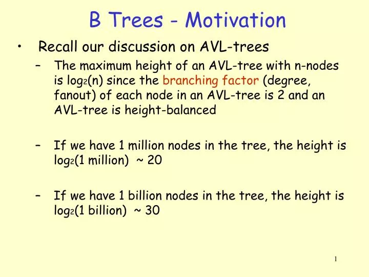
B Trees - Motivation • Recall our discussion on AVL-trees • The maximum height of an AVL-tree with n-nodes is log2(n) since the branching factor (degree, fanout) of each node in an AVL-tree is 2 and an AVL-tree is height-balanced • If we have 1 million nodes in the tree, the height is log2(1 million) ~ 20 • If we have 1 billion nodes in the tree, the height is log2(1 billion) ~ 30
B Trees - Motivation • To reach an item residing at the deepest level • Have to visit 20/30 nodes starting at the root • What if the tree nodes do not fit into memory • Will be the case if we have millions of nodes in the tree • Then we have to retrieve the visited nodes from the disk • Disk access is very slow • Each block retrieval takes ~ 20ms from a hard-disk. Retrieving 20 nodes will take ~4 seconds. • Solution? B Trees • Increase the branching factor of nodes while keeping the tree balanced so that the height of the tree will be small • If branching factor is 10, then the height is log10(1 billion) = 9, if the branching factor is 100, then the height is log100(1 billion) = 5
B Trees • B-Trees are multi-way search trees commonly used in database systems or other applications where data is stored externally on disks and keeping the tree shallow is important. • A B-Tree of order M has the following properties: • The root is either a leaf or has between 2 and M children. • All nonleaf nodes (except the root) have between |M/2| and M children. • All leaves are at the same depth.
B Trees • Several variations on the general idea • The actual data is stored in both the leaves and the internal nodes • This is typically called the B tree in literature • The actual data is stored ONLY at the leaves. Internal nodes ONLY contain keys to guide the search to the actual data stored at the leaves • This is what your book calls the B tree. But this version is typically called the B+ tree in literature • We will cover this version in this class
B Trees • A B Tree of order M has the following properties: • The root is either a leaf or has between 2 and M children. • All nonleaf nodes (except the root) have between |M/2| and M children. • All leaves are at the same depth. • All data records are stored at the leaves. • Leaves store between |L/2| and L data records. • L depends on disk block size and data record size (e.g. L = M).
B Tree Details • Each internal node of a B-tree has: • Between |M/2| and M children. • up to M-1 keys k1 < k2 < ... < kM-1 k1 ….. ki-1 ki …….kM-1 Keys are ordered so that: k1 < k2 < ... < kM-1
Properties of B-Trees k1 ….. ki-1 ki …….kM-1 T1 TM Ti • Children of each internal node are "between" the items in that node. • Suppose subtree Ti is the ith child of the node: • All keys in Ti must be between ki-1 and ki • i.e. ki-1 ≤ Ti < ki • ki-1 is the smallest key in Ti • All keys in first subtree T1< k1 • All keys in last subtree TM ≥ kM-1
B-Tree Example • B-tree of order 3: also known as 2-3 tree (2 to 3 children) - means empty key 22: - 16: - 41: 58 16, 17 58, 59, 61 8, 11, 12 41, 52 22, 23, 31 • Apply B-tree definition for order M = 3 and L = M = 3 • Each node must have at least |M/2| = 2 and at most M = 3 children • Leaves store between |L/2| = 2 and L = 3 data records
Searching for a key in the B tree • Searching a B-tree is much like searching a binary-tree, except that instead of making a “two-way” branching decision at each node, we make a “multi-way” branching decision according to the number of the node’s children. Search for 52 in the following 2-3 tree 22: - 16: - 41: 58 16, 17 58, 59, 61 8, 11, 12 41, 52 22, 23, 31
Inserting Items in B Trees • Insert X: Do a Search on X and find appropriate leaf node • If leaf node is not full, fill in empty slot with X. 22: - 16: - 41: 58 16, 17 58, 59, 61 8, 11, 12 41, 52 22, 23, 31 Insert 18 22: - 16: - 41: 58 16, 17, 18 58, 59, 61 8, 11, 12 41, 52 22, 23, 31
Inserting Items in B Trees • Insert X: Do a Search on X and find appropriate leaf node • If leaf node is full, split leaf node and adjust parents up to root node. 22: - 16: - 41: 58 16, 17, 18 58, 59, 61 8, 11, 12 41, 52 22, 23, 31 Insert 1 22: - 11: 16 41: 58 1, 8 11, 12 16, 17, 18 58, 59, 61 41, 52 22, 23, 31
Insertion in B Trees: Insert 19 22: - 11: 16 41: 58 1, 8 11, 12 16, 17, 18 58, 59, 61 41, 52 22, 23, 31 Insert 19 22: - 11: 16 41: 58 1, 8 11, 12 16, 17 58, 59, 61 18, 19 41, 52 22, 23, 31 Split (11:16)
Insertion in B Trees: Insert 28 Split (11:16) into 2 nodes (11: -) and (18: -) Push 16 to the root 16: 22 11: - 18: - 41: 58 58, 59, 61 41, 52 22, 23, 31 1, 8 11, 12 16, 17 18, 19 Insert 28: Split (22, 23, 31) into 2 nodes 16: 22 11: - 18: - 41: 58 58, 59, 61 41, 52 22, 23 28, 31 1, 8 11, 12 16, 17 18, 19
Insertion in B Trees: Insert 28 Insert 28: Split (28:41:58) into 2 nodes (28: -) and (58: -) and push 41 to the root 16: 22 11: - 18: - 58: - 28: - 58, 59, 61 16, 17 41, 52 18, 19 1, 8 11, 12 22, 23 28, 31 Can’t insert 41 to the root: Split the root, (16:22:41) into two nodes (16: -), (41: -), create a new root and push 22 to the new root 22: - 16: - 41: - 11: - 18: - 58: - 28: - 58, 59, 61 16, 17 41, 52 18, 19 1, 8 11, 12 22, 23 28, 31
Pseudocode for Btree Insert • Search the Btree and find the leaf node where the key will be inserted • If the leaf has enough space, insert the key into the leaf and your are done • Otherwise, split the leaf into 2 leaves. Now you have a (key, child) pair that needs to be inserted into the parent • If parent has enough space, insert • Otherwise split the parent, and propagate this process up in the tree
Deleting Items from B Trees • Delete X: Do a Search on X and delete the value from leaf node • May have to combine leaf nodes and adjust parents up to root node if number of data items falls below |L/2| = 2 • E.g. Delete 59 in the tree below – Case 1 – Simple case 16: 22 11: - 18: - 41: 58 58, 59, 61 41, 52 22, 23, 31 1, 8 11, 12 16, 17 18, 19 Delete 59
Deletion in B Trees: Delete 52 16: 22 11: - 18: - 41: 58 58, 61 41, 52 22, 23, 31 1, 8 11, 12 16, 17 18, 19 Delete 52: Leaf (41,-) has a single key. But Left sibling has 3 keys. So borrow 1 key from the sibling – Case 2 16: 22 11: - 18: - 31: 58 58, 61 31, 41 22, 23 1, 8 11, 12 16, 17 18, 19
Deletion in B Trees: Delete 41 16: 22 11: - 18: - 31: 58 58, 61 31, 41 22, 23 1, 8 11, 12 16, 17 18, 19 Delete 41: Node (31, 41) now has (31: -). We can’t borrow from any of the siblings. So we combine with one of them 16: 22 11: - 18: - 58: - 22, 23, 31 1, 8 58, 61 11, 12 16, 17 18, 19
Deletion in B Trees: Delete 17 16: 22 11: - 18: - 58: - 22, 23, 31 1, 8 58, 61 11, 12 16, 17 18, 19 Delete 17: Node now has (16: -). Must Combine with (18, 19). Now the parent has A single child! So must combine the siblings 22: - 11: 16 31: - 16, 18, 19 1, 8 11, 12 22, 23, 31 58, 61
Pseudocode for Btree Delete • Search the Btree and find the leaf node containing the key, and delete the key from the leaf • If the leaf still has enough keys, your are done • Otherwise, try borrowing from the right OR left siblings. If this is possible, then you are done • Otherwise, merge with the right OR left sibling. Now the porent has one less child. • If the parent still has enough children you are done. Otherwise, apply the same procedure to this internal node, and propagate the process up the tree
Choosing M and L Parameters • If Tree & Data in internal (main) memory • We want M and L to be small to minimize search time at each node/leaf • Typically M = 3 or 4 (e.g. M = 3 is a 2-3 tree) • All N items stored in internal memory • If Tree & Data on Disk then Disk access time dominates! • Choose M & L so that interior and leaf nodes fit on 1 disk block • To minimize number of disk accesses, minimize tree height • Typically M = 32 to 256, so that depth = 2 or 3 allows very fast access to data in large databases.
Efficient Range Searches with B Trees • Consider the following database query • Find all students whose keys are between ID1 and ID2 • Find all records whose keys are between “G and R” • Find all cities whose names start with D • …
Efficient Range Searches with B Trees • To solve range queries efficiently, the leaves of a B tree are typically linked together in a doubly linked list as shown below 22: - 16: - 41: - 11: - 18: - 58: - 28: - 58, 59, 61 16, 17 41, 52 18, 19 1, 8 11, 12 22, 23 28, 31
Efficient Range Searches with B Trees • Find all records whose keys are between “16 and 28” • Do a search to find “16” within the leaf node “16, 17” • Then simply follow the links to the adjacent leafs until we hit the leaf containing “28” • Notice that we only accessed 3 internal and 4 leaf nodes to execute the whole query. 22: - 16: - 41: - 11: - 18: - 58: - 28: - 58, 59, 61 16, 17 41, 52 18, 19 1, 8 11, 12 22, 23 28, 31
The height of a B tree • If n >= 1, then for any n-key B-tree T of height h and minimum degree |M/2| = t >=2, • Proof: If a B-tree has height h, the root contains at least one key and all other nodes contain at least t-1 keys. Thus, • there is one node at depth 0, which is the root • there are at least 2 nodes at depth 1 • at least 2t nodes at depth 2 • at least 2t2 nodes ad depth 3 and so on • until at depth “h” there are at least 2t(h-1) nodes. • Let’s look at the next slide for an illustration of the above statement.
t-1 t-1 t-1 t-1 t-1 t-1 t-1 t-1 t-1 t-1 t-1 t-1 1 t-1 t-1 The height of a B tree # of nodes • A B-tree of height 3 containing a minimum possible number of keys. Shown inside each node x is |M/2|-1, that is, the # of keys contained within the node. root 1 2 t t 2t ………… …………. t t t 2t2 t …. …. …. ….
Summary of Search Trees • Binary Search Trees: Allow faster search compared to linear linked lists. But the shape of the tree depends on the order of insertion. So the tree might degenerate to a linked list. • AVL trees: Insert/Delete operations keep tree balanced. Complicated insertion/deletion. Extra space for balancing factor • Splay trees: Sequence of operations produces more-or-less balanced trees. Active nodes move up the tree, which allows for faster access next time they are accessed • Multi-way search trees (B, B+ Trees): More than two children per node allows shallow trees; all leaves are at the same depth keeping tree balanced at all times. Good for huge data sets and used in database management systems, where the data does not fit in main memory and stored on disk.