Download
1 / 55
550 likes | 792 Views
Chapter 4 (4.1-4.3). Informed Search and Exploration. Introduction. Ch.3 searches – good building blocks for learning about search But vastly inefficient eg: Can we do better?. (Quick Partial) Review. Previous algorithms differed in how to select next node for expansion eg:

E N D
Chapter 4 (4.1-4.3) Informed Search and Exploration
Introduction • Ch.3 searches – good building blocks for learning about search • But vastly inefficient eg: • Can we do better?
(Quick Partial) Review • Previous algorithms differed in how to select next node for expansion eg: • Breadth First • Fringe nodes sorted old -> new • Depth First • Fringe nodes sorted new -> old • Uniform cost • Fringe nodes sorted by path cost: small -> big • Used little (no) “external” domain knowledge
Overview • Heuristic Search • Best-First Search Approach • Greedy • A* • Heuristic Functions • Local Search and Optimization • Hill-climbing • Simulated Annealing • Local Beam • Genetic Algorithms
Informed Searching • An informed search strategy uses knowledge beyond the definition of the problem • The knowledge is embodied in an evaluation function f(n)
Best-First Search • An algorithm in which a node is selected for expansion based on an evaluation function f(n) • Fringe nodes ordered by f(n) • Traditionally the node with the lowest evaluation function is selected • Not an accurate name…expanding the best node first would be a straight march to the goal. • Choose the node that appears to be the best
Best-First Search • Remember: Uniform cost search • F(n) = g(n) • Best-first search: • F(n) = h(n) • Later, a-star search: • F(n) = g(n) + h(n)
Best-First Search (cont.) • Some BFS algorithms also include the notion of a heuristic function h(n) • h(n) = estimated cost of the cheapest path from node n to a goal node • Best way to include informed knowledge into a search • Examples: • How far is it from point A to point B • How much time will it take to complete the rest of the task at current node to finish
Greedy Best-First Search • Expands node estimated to be closest to the goal • f(n) = h(n) • Consider the route finding problem. • Can we use additional information to avoid costly paths that lead nowhere? • Consider using the straight line distance (SLD)
Route Finding 374 253 366 329
Route Finding: Greedy Best First Arad f(n) = 366
Sibiu Timisoara Zerind 253 329 374 Route Finding: Greedy Best First Arad f(n) = 366
Sibiu Timisoara Zerind 253 329 374 Arad Fagaras Oradea Rimnicu Vilcea 366 176 380 193 Route Finding: Greedy Best First Arad f(n) = 366
Sibiu Timisoara Zerind 253 329 374 Arad Fagaras Oradea Rimnicu Vilcea 366 176 380 193 Bucharest Sibiu 0 253 Route Finding: Greedy Best First Arad f(n) = 366
Exercise So is Arad->Sibiu->Fagaras->Bucharest optimal?
Greedy Best-First Search • Not optimal. • Not complete. • Could go down a path and never return to try another. • e.g., Iasi Neamt Iasi Neamt … • Space Complexity • O(bm) – keeps all nodes in memory • Time Complexity • O(bm) (but a good heuristic can give a dramatic improvement)
Example: 8-Puzzle Average solution cost for a random puzzle is 22 moves Branching factor is about 3 Empty tile in the middle -> four moves Empty tile on the edge -> three moves Empty tile in corner -> two moves 322 is approx 3.1e10 Get rid of repeated states 181,440 distinct states Heuristic Functions
Heuristic Functions • h1 = number of misplaced tiles • h2 = sum of distances of tiles to goal position.
Heuristic Functions • h1 = 7 • h2 = 4+0+3+3+1+0+2+1 = 14
Admissible Heuristics • A heuristic function h(n) is admissible if it never overestimates the cost to reach the goal from n • Another property of heuristic functions is consistency • h(n) c(n,a,n’) + h(n’) where: • c(n,a,n’) is the cost to get to n’ from n using action a. • Consistent h(n) the values of f(n) along any path are non-decreasing • Graph search is optimal if h(n) is consistent
Heuristic Functions • Is h1 (#of displaced tiles) • admissible? • consistent? • Is h2 (Manhattan distance) • admissible? • consistent?
Dominance • If h2(n) ≥ h1(n) for all n (both admissible) • then h2dominatesh1 • h2is better for search • Typical search costs (average number of nodes expanded): • d=12 IDS = 3,644,035 nodes A*(h1) = 227 nodes A*(h2) = 73 nodes • d=24 IDS = too many nodes A*(h1) = 39,135 nodes A*(h2) = 1,641 nodes
Heuristic Functions • Heuristics are often obtained from relaxed problem • Simplify the original problem by removing constraints • The cost of an optimal solution to a relaxed problem is an admissible heuristic.
8-Puzzle • Original • A tile can move from A to B if A is horizontally or vertically adjacent to B and B is blank. • Relaxations • Move from A to B if A is adjacent to B(remove “blank”) • h2 by moving each tile in turn to destination • Move from A to B (remove “adjacent” and “blank”) • h1 by simply moving each tile directly to destination
How to Obtain Heuristics? • Ask the domain expert (if there is one) • Solve example problems and generalize your experience on which operators are helpful in which situation (particularly important for state space search) • Try to develop sophisticated evaluation functions that measure the closeness of a state to a goal state (particularly important for state space search) • Run your search algorithm with different parameter settings trying to determine which parameter settings of the chosen search algorithm are “good” to solve a particular class of problems. • Write a program that selects “good parameter” settings based on problem characteristics (frequently very difficult) relying on machine learning
A* Search • The greedy best-first search does not consider how costly it was to get to a node. • f(n) = h(n) • Idea: avoid expanding paths that are already expensive • Combine g(n), the cost to reach node n, with h(n) • f(n) = g(n) + h(n) • estimated cost of cheapest solution through n
A* Search • When h(n) = actual cost to goal • Only nodes in the correct path are expanded • Optimal solution is found • When h(n) < actual cost to goal • Additional nodes are expanded • Optimal solution is found • When h(n) > actual cost to goal • Optimal solution can be overlooked
A* Search • Complete • Yes, unless there are infinitely many nodes with f <= f(G) • Time • Exponential in [relative error of h x length of soln] • The better the heuristic, the better the time • Best case h is perfect, O(d) • Worst case h = 0, O(bd) same as BFS • Space • Keeps all nodes in memory and save in case of repetition • This is O(bd) or worse • A* usually runs out of space before it runs out of time • Optimal • Yes, cannot expand fi+1 unless fi is finished
Sibiu Timisoara Zerind 393 =140+253 447 449 Arad Fagaras Oradea Rimnicu Vilcea 646 415 671 413 A* Search Arad f(n) = 0 + 366 Things are different now!
Bucharest Sibiu Craiova Pitesti Sibiu 526 450 591 417 553 Bucharest Craiova Rimnicu Vilcea 615 418 607 A* Search Continued Arad Fagaras Oradea Rimnicu Vilcea 646 415 671 413
A* Search; complete • A* is complete. • A* builds search “bands” of increasing f(n) • At all points f(n) < C* • Eventually we reach the “goal contour” • Optimally efficient • Most times exponential growth occurs
Memory Bounded Heuristic Search • Ways of getting around memory issues of A*: • IDA* (iterative deepening algorithm) • Cutoff = f(n) instead of depth • Recursive Best First Search • Mimic standard BFS, but use linear space! • Keeps track of best f(n) from alternate paths • Disad’s: excessive node regeneration from recursion • Too little memory! use memory-bounded approaches • Cutoff when memory bound is reached and other constraints
Local Search / Optimization • Idea is to find the best state. • We don’t really care how to get to the best state, just that we get there. • The best state is defined according to an objective function • Measures the “fitness” of a state. • Problem: Find the optimal state • The one that maximizes (or minimizes) the objective function.
State Space Landscapes Objective Function global max local max shoulder State Space
Problem Formulation • Complete-state formulation • Start with an approximate solution and perturb • n-queens problem • Place n queens on a board so that no queen is attacking another queen.
Problem Formulation • Initial State: n queens placed randomly on the board, one per column. • Successor function: States that obtained by moving one queen to a new location in its column. • Heuristic/objective function: The number of pairs of attacking queens.
n-Queens 4 4 4 4 3 5 2 5 4 2 3 3 2 5 3 5 2 3 2 1 3 3 2 4
Local Search Algorithms • Hill climbing • Simulated annealing • Local beam search • Genetic Algorithms
Objective Function State Space Hill Climbing (or Descent)
Hill Climbing Pseudo-code • "Like climbing Everest in thick fog with amnesia"
Objective Function State Space Hill Climbing Problems
n-Queens 4 4 4 4 3 5 2 5 4 2 3 3 2 5 3 5 2 3 2 1 3 3 2 4 What happens if we move 3rd queen?
Possible Improvements • Stochastic hill climbing • Choose at random from uphill moves • Probability of move could be influenced by steepness • First-choice hill climbing • Generate successors at random until one is better than current. • Random-restart • Execute hill climbing several times, choose best result. • If p is probability of a search succeeding, then expected number of restarts is 1/p.
Simulated Annealing • Similar to stochastic hill climbing • Moves are selected at random • If a move is an improvement, accept • Otherwise, accept with probability less than 1. • Probability gets smaller as time passes and by the amount of “badness” of the move.
Simulated Annealing Algorithm Success
Traveling Salesperson Problem • Tour of cities • Visit each one exactly once • Minimize distance/cost/etc.
Local Beam Search • Keep k states in memory instead of just one • Generate successors of all k states • If one is a goal, return the goal • Otherwise, take k best successors and repeat.