Download
1 / 41
480 likes | 770 Views
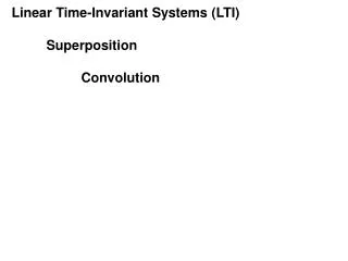
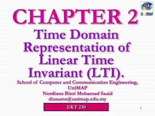
2. CHAPTER. Time-Domain Representations of LTI Systems. 2.1 Introduction. Objectives: Impulse responses of LTI systems Linear constant-coefficients differential or difference equations of LTI systems Block diagram representations of LTI systems State-variable descriptions for LTI systems.

E N D
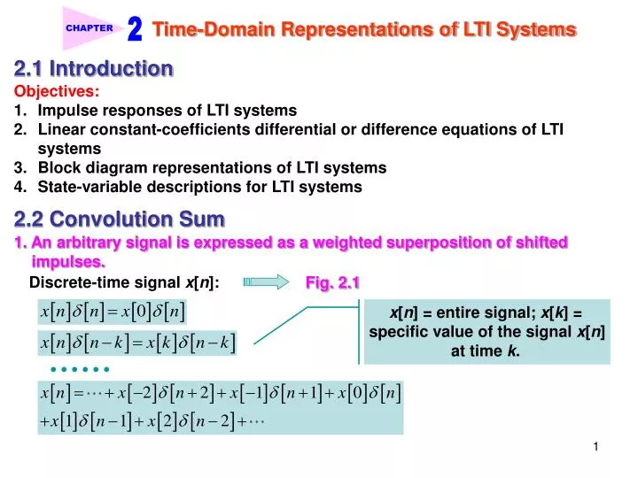
2 CHAPTER Time-Domain Representations of LTI Systems 2.1 Introduction • Objectives: • Impulse responses of LTI systems • Linear constant-coefficients differential or difference equations of LTI systems • Block diagram representations of LTI systems • State-variable descriptions for LTI systems 2.2 Convolution Sum 1. An arbitrary signal is expressed as a weighted superposition of shifted impulses. Discrete-time signal x[n]: Fig. 2.1 x[n] = entire signal; x[k] = specific value of the signal x[n] at time k.
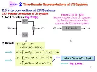
2 CHAPTER Input x[n] Output y[n] LTI system H Time-Domain Representations of LTI Systems Figure 2.1 (p. 99)Graphical example illustrating the representation of a signal x[n] as a weighted sum of time-shifted impulses. (2.1) 2. Impulse response of LTI system H: Output: Linearity Linearity (2.2)
2 CHAPTER Time-Domain Representations of LTI Systems The system output is a weighted sum of the response of the system to time- shifted impulses. For time-invariant system: h[n] = H{[n]} impulse response of the LTI system H (2.3) (2.4) Convolution process: Fig. 2.2. 3. Convolution sum: Figure 2.2a (p. 100)Illustration of the convolution sum. (a) LTI system with impulse response h[n] and input x[n].
2 CHAPTER Time-Domain Representations of LTI Systems Figure 2.2b (p. 101)(b) The decomposition of the input x[n] into a weighted sum of time-shifted impulses results in an output y[n] given by a weighted sum of time-shifted impulse responses. d
2 CHAPTER Time-Domain Representations of LTI Systems The output associated with the kth input is expressed as: Example 2.1Multipath Communication Channel: Direct Evaluation of the Convolution Sum Consider the discrete-time LTI system model representing a two-path propagation channel described in Section 1.10. If the strength of the indirect path is a = ½, then Letting x[n] = [n], we find that the impulse response is
2 CHAPTER time-shifted impulse input time-shifted impulse response output [n k] h[nk] Time-Domain Representations of LTI Systems Determine the output of this system in response to the input Input = 0 for n < 0 and n > 0 <Sol.> 1. Input: 2. Since 3. Output: (convolution of x[n] and h[n])
2 CHAPTER Time-Domain Representations of LTI Systems 2.3 Convolution Sum Evaluation Procedure 1. Convolution sum: k = independent variable 2. Define the intermediate signal: (2.5) n is treated as a constant by writing n as a subscript on w. h[nk] = h [ (k n)] is a reflected (because of k) and time-shifted (by n) version of h [k]. 3. Since The time shift n determines the time at which we evaluate the output of the system. (2.6) Example 2.2Convolution Sum Evaluation by using Intermediate Signal Consider a system with impulse response Use Eq. (2.6) to determine the output of the system at time n = 5, n = 5, and n = 10 when the input is x [n] = u [n].
2 CHAPTER Time-Domain Representations of LTI Systems <Sol.> Fig. 2.3 depicts x[k] superimposed on the reflected and time-shifted impulse response h[n k]. 1. h [n k]=(3/4)n-ku[n-k] For n = 10: 2. Intermediate signal wn[k]: For n = 5: (x[k]=u[k]=0, k<=-5=n) Eq. (2.6) y[ 5] = 0 Eq. (2.6) For n = 5: Eq. (2.6)
2 CHAPTER Time-Domain Representations of LTI Systems Figure 2.3 (p. 103) Evaluation of Eq. (2.6) in Example 2.2. (a) The input signal x[k] above the reflected and time-shifted impulse response h[n – k], depicted as a function of k. (b) The product signal w5[k] used to evaluate y [–5]. (c) The product signal w5[k] used to evaluate y[5]. (d) The product signal w10[k] used to evaluate y[10].
2 CHAPTER Time-Domain Representations of LTI Systems Procedure 2.1: Reflect and Shift Convolution Sum Evaluation 1. Graph both x[k] and h[n k] as a function of the independent variable k. To determine h[nk] , first reflect h[k] about k = 0 to obtain h[k]. Then shift by n. 2. Begin with n large and negative. That is, shift h[ k] to the far left on the time axis. 3. Write the mathematical representation for the intermediate signal wn[k]. 4. Increase the shift n (i.e., move h[nk] toward the right) until the mathematical representation for wn[k] changes. The value of n at which the change occurs defines the end of the current interval and the beginning of a new interval. 5. Let n be in the new interval. Repeat step 3 and 4 until all intervals of times shifts and the corresponding mathematical representations for wn[k] are identified. This usually implies increasing n to a very large positive number. 6. For each interval of time shifts, sum all the values of the corresponding wn[k] to obtain y[n] on that interval.
2 CHAPTER Time-Domain Representations of LTI Systems Example 2.3Moving-Average System: Reflect-and-shift Convolution Sum Evaluation The output y[n] of the four-point moving-average system is related to the input x[n] according to the formula The impulse response h[n] of this system is obtained by letting x[n] = [n], which yields Fig. 2.4 (a). Determine the output of the system when the input is the rectangular pulse defined as 1’st interval: n < 0 2’nd interval: 0 ≤ n ≤ 3 3’rd interval: 3 <n ≤ 9 4th interval: 9 < n ≤ 12 5th interval: n > 12 Fig. 2.4 (b). <Sol.> 1. Refer to Fig. 2.4. Five intervals ! 2. 1’st interval: wn[k] = 0 3. 2’nd interval: Fig. 2.4 (c). For n = 0:
2 CHAPTER Time-Domain Representations of LTI Systems Figure 2.4 (p. 106)Evaluation of the convolution sum for Example 2.3. (a) The system impulse response h[n]. (b) The input signal x[n]. (c) The input above the reflected and time-shifted impulse response h[n – k], depicted as a function of k. (d) The product signal wn[k] for the interval of shifts 0 n 3. (e) The product signal wn[k] for the interval of shifts 3 < n 9. (f) The product signal wn[k] for the interval of shifts 9 < n 12. (g) The output y[n].
2 CHAPTER Time-Domain Representations of LTI Systems 6. 5th interval: n > 12 wn[k] = 0 For n = 1: 7. Output: The output of the system on each interval n is obtained by summing the values of the corresponding wn[k] according to Eq. (2.6). For general case: n 0: 1) For n < 0 and n > 12: y[n] = 0. Fig. 2.4 (d). 2) For 0 ≤ n≤ 3: 4. 3’rd interval: 3 < n≤ 9 Fig. 2.4 (g) 3) For 3 < n ≤ 9: Fig. 2.4 (e). 5. 4th interval: 9 < n ≤ 12 4) For 9 < n ≤ 12: Fig. 2.4 (f).
2 CHAPTER Time-Domain Representations of LTI Systems Example 2.4First-order Recursive System: Reflect-and-shift Convolution Sum Evaluation The input-output relationship for the first-order recursive system is given by Let the input be given by We use convolution to find the output of this system, assuming that b and that the system is causal. <Sol.> 1. Impulse response: (2.7) Since the system is causal, we have h[n] = 0 for n < 0 (why?). For n = 0, 1, 2, …, we find that h[0] = 1, h[1] = , h[2] = 2, …, or 2. Graph of x[k] and h[n k]: Fig. 2.5 (a). and 3. Intervals of time shifts: 1’st interval: n < 4; 2’nd interval: n 4
2 CHAPTER Time-Domain Representations of LTI Systems Figure 2.5a&b (p. 109) Evaluation of the convolution sum for Example 2.4. (a) The input signal x[k] depicted above the reflected and time-shifted impulse response h[n – k]. (b) The product signal wn[k] for –4 n.
2 CHAPTER Time-Domain Representations of LTI Systems 4. For n < 4: wn[k] = 0. Next, we apply the formula for summing a geometric series of n + 5 terms to obtain 5. For n 4: Fig. 2.5 (b). 6. Output: Combining the solutions for each interval of time shifts gives the system output: 1) For n < 4: y[n] = 0. 2) For n 4: Fig. 2.5 (c). Let m = k + 4, then Assuming that = 0.9 and b = 0.8.
2 CHAPTER Time-Domain Representations of LTI Systems Figure 2.5c (p. 110)(c) The output y[n] assuming that p = 0.9 and b = 0.8.
2 CHAPTER Time-Domain Representations of LTI Systems Example 2.5Investment Computation The first-order recursive system is used to describe the value of an investment earning compound interest at a fixed rate of r % per period if we set = 1 + (r/100). Let y[n] be the value of the investment at the start of period n. If there are no deposits or withdrawals, then the value at time n is expressed in terms of the value at the previous time as y[n] = y[n 1]. Now, suppose x[n] is the amount deposited (x[n] > 0) or withdrawn (x[n] < 0) at the start of period n. In this case, the value of the amount is expressed by the first-order recursive equation We use convolution to find the value of an investment earning 8 % per year if $1000 is deposited at the start of each year for 10 years and then $1500 is withdrawn at the start each year for 7 years. <Sol.> 1. Prediction: Account balance to grow for the first 10 year, and to decrease during next 7 years, and afterwards to continue growing. 2. By using the reflect-and-shift convolution sum evaluation procedure, we can evaluate y[n] = x[n] h[n], where x[n] is depicted in Fig. 2.6 and h[n] = nu[n] is as shown in Example 2.4 with = 1.08.
2 CHAPTER Time-Domain Representations of LTI Systems Figure 2.6 (p. 111)Cash flow into an investment. Deposits of $1000 are made at the start of each of the first 10 years, while withdrawals of $1500 are made at the start of each of the second 10 years. 3. Graphs of x[k] and h[n k]: Fig. 2.7(a). 4. Intervals of time shifts: 1’st interval: n < 0 2’nd interval: 0 ≤ n ≤ 9 3’rd interval: 10 ≤n ≤ 16 4th interval: 17 ≤ n 5. Mathematical representations for wn[k] and y[n]: 1) For n < 0: wn[k] = 0 and y[n] = 0
2 CHAPTER Time-Domain Representations of LTI Systems Figure 2.7a-d (p. 111)Evaluation of the convolution sum for Example 2.5. (a) The input signal x[k] depicted above the reflected and time-shifted impulse response h(n – k). (b The product signal wn[k] for 0 n 9. (c) The product signal wn[k] for 10 n 16. (d) The product signal wn[k] for 17 n.
2 CHAPTER Time-Domain Representations of LTI Systems 2) For 0 ≤ n≤ 9: Fig. 2.7 (b). Apply the formula for summing a geometric series 3) For 10 ≤ n ≤ 16: Fig. 2.7 (c).
2 CHAPTER Time-Domain Representations of LTI Systems m = k 10 Apply the formula for summing a geometric series 4) For 17 ≤ n : Fig. 2.7 (d).
2 CHAPTER Time-Domain Representations of LTI Systems 6. Fig. 2,7(e) depicts y[n], the value of the investment at the start of each period, by combining the results for each of the four intervals. Figure 2.7e (p. 113)(e) The output y[n] representing the value of the investment immediately after the deposit or withdrawal at the start of year n.
2 CHAPTER Input x(t) Output y(t) LTI system H Time-Domain Representations of LTI Systems 2.4 The Convolution Integral 1. A continuous-time signal can be expressed as a weighted superposition of time-shifted impulses. The sifting property of the impulse ! (2.10) 2. Impulse response of LTI system H: Output: Linearity property (2.10) 3. h(t) = H{(t)} impulse response of the LTI system H If the system is also time invariant, then A time-shifted impulse generates a time-shifted impulse response output (2.11) (2.12) Fig. 2.9.
2 CHAPTER Time-Domain Representations of LTI Systems Convolution integral: 2.5 Convolution Integral Evaluation Procedure 1. Convolution integral: (2.13) 2. Define the intermediate signal: = independent variable, t = constant h (t) = h ( ( t)) is a reflected and shifted (by t) version of h(). 3. Output: The time shift t determines the time at which we evaluate the output of the system. (2.14)
2 CHAPTER Time-Domain Representations of LTI Systems Procedure 2.2: Reflect and Shift Convolution Integral Evaluation 1. Graph both x() and h(t) as a function of the independent variable . To obtain h(t), reflect h()about = 0 to obtain h( ) and then h( )shift by t. 2. Begin with the shift t large and negative. That is, shift h( )to the far left on the time axis. 3. Write the mathematical representation for the intermediate signal wt (). 4. Increase the shift t (i.e., move h(t)toward the right) until the mathematical representation for wt () changes. The value of t at which the change occurs defines the end of the current set and the beginning of a new set. 5. Let t be in the new set. Repeat step 3 and 4 until all sets of shifts t and the corresponding mathematical representations for wt () are identified. This usually implies increasing t to a very large positive number. 6. For each sets of shifts t, integrate wt () from = to = to obtain y(t). Example 2.6Reflect-and-shift Convolution Evaluation Given and as depicted in Fig. 2-10, Evaluate the convolution integral y(t) = x(t) h(t).
2 CHAPTER Time-Domain Representations of LTI Systems Figure 2.10 (p. 117)Input signal and LTI system impulse response for Example 2.6. <Sol.> 1. Graph of x() and h(t): Fig. 2.11 (a). 2. Intervals of time shifts: Four intervals 1’st interval: t < 1 2’nd interval: 1 ≤ t < 3 3’rd interval: 3 ≤ t < 5 4th interval: 5 ≤ t wt() = 0 3. First interval of time shifts: t < 1 4. Second interval of time shifts: 1 ≤ t < 3 Fig. 2.11 (b).
2 CHAPTER Time-Domain Representations of LTI Systems Figure 2.11 (p. 118)Evaluation of the convolution integral for Example 2.6. (a) The input x() depicted above the reflected and time-shifted impulse response. (b) The product signal wt() for 1 t < 3. (c) The product signal wt() for 3 t < 5. (d) The system output y(t). t
2 CHAPTER Time-Domain Representations of LTI Systems 5. Third interval: 3 ≤ t < 5 Fig. 2.11 (c). wt() = 0 6. Fourth interval: 5 ≤ t 7. Convolution integral: 1) For t < 1 and t 5: y(t) = 0 2) For second interval 1 ≤ t < 3, y(t) = t 1 3) For third interval 3 ≤ t < 5, y(t) = 3 (t 2) Figure 2.12 (p. 119)RC circuit system with the voltage source x(t) as input and the voltage measured across the capacitor y(t), as output. Example 2.7RC Circuit Output For the RC circuit in Fig. 2.12, assume that the circuit’s time constant is RC = 1 sec. Ex. 1.21 shows that the impulse response of this circuit is h(t) = e tu(t). Use convolution to determine the capacitor voltage, y(t), resulting from an input voltage x(t) = u(t) u(t 2).
2 CHAPTER Time-Domain Representations of LTI Systems <Sol.> RC circuit is LTI system, so y(t) = x(t) h(t). 1. Graph of x() and h(t): Fig. 2.13 (a). and 2. Intervals of time shifts: Three intervals 1’st interval: t < 0 2’nd interval: 0 ≤ t < 2 3’rd interval: 2 ≤t wt() = 0 3. First interval of time shifts: t < 0 4. Second interval of time shifts: 0 ≤ t < 2 For t > 0, Fig. 2.13 (b). 5. Third interval: 2 ≤ t Fig. 2.13 (c).
2 CHAPTER Time-Domain Representations of LTI Systems Figure 2.13 (p. 120)Evaluation of the convolution integral for Example 2.7. (a) The input x() superimposed over the reflected and time-shifted impulse response h(t – ), depicted as a function of . (b) The product signal wt() for 0t < 2. (c) The product signal wt() for t 2. (d) The system output y(t). t
2 CHAPTER Time-Domain Representations of LTI Systems 6. Convolution integral: 1) For t < 0: y(t) = 0 2) For second interval 0 ≤ t < 2: 3) For third interval 2 ≤ t: Fig. 2.13 (d). Example 2.8Another Reflect-and-Shift Convolution Evaluation Suppose that the input x(t) and impulse response h(t) of an LTI system are, respectively, given by and Find the output of the system.
2 CHAPTER Time-Domain Representations of LTI Systems <Sol.> 1. Graph of x() and h(t): Fig. 2.14 (a). 2. Intervals of time shifts: Five intervals 1’st interval: t < 0 2’nd interval: 0 ≤ t < 2 3’rd interval: 2 ≤t < 3 4th interval: 3 ≤ t < 5 5th interval: t 5 wt() = 0 3. First interval of time shifts: t < 0 4. Second interval of time shifts: 0 ≤ t < 2 Fig. 2.14 (b). 5. Third interval of time shifts: 2 ≤ t < 3 Fig. 2.14 (c). 6. Fourth interval of time shifts: 3 ≤ t < 5
2 CHAPTER Time-Domain Representations of LTI Systems Figure 2.14 (p. 121) Evaluation of the convolution integral for Example 2.8. (a) The input x() superimposed on the reflected and time-shifted impulse response h(t – ), depicted as a function of . (b) The product signal wt() for 0 t < 2. (c) The product signal wt() for 2 t < 3. (d) The product signal wt() for 3 t < 5. (e) The product signal wt() for t 5. The system output y(t). t
2 CHAPTER Time-Domain Representations of LTI Systems Fig. 2.14 (d). 7. Fifth interval of time shifts: t 5 Fig. 2.14 (e). 8. Convolution integral: 1) For t < 0: y(t) = 0 2) For second interval 0 ≤ t < 2: 3) For third interval 2 ≤ t < 3:y(t) = 2 4) For third interval 3 ≤ t < 5: 5) For third interval t 5: y(t) = 2
2 CHAPTER Time-Domain Representations of LTI Systems Fig. 2.14 (f). Example 2.9Radar range Measurement: Propagation Model We identify an LTI system describing the propagation of the pulse. Let the transmitted RF pulse be given by as shown in Fig. 2.16 (a). Suppose we transmit an impulse from the radar to determine the impulse response of the round-trip propagation to the target. The impulse is delay in time and attenuated in amplitude, which results in the impulse response h(t) = a(t ), where a represents the attenuation factor and the round-trip time delay. Use the convolution of x(t) with h(t) to verify this result.
2 CHAPTER Time-Domain Representations of LTI Systems <Sol.> 1. Find h(t ): Reflectingh(t) = a (t) about = 0 gives h() = a(+), since the impulse has even symmetry. 2. Shift the independent variable by t to obtain h(t ) = a ( (t)). 3. Substitute this equation for h(t) into the convolution integral of Eq. (2.12), and use the shifting property of the impulse to obtain the received signal as Figure 2.16 (p. 124)Radar range measurement. (a) Transmitted RF pulse. (b) The received echo is an attenuated and delayed version of the transmitted pulse.
2 CHAPTER Time-Domain Representations of LTI Systems Example 2.10Radar range Measurement (continued): The Matched Filter In Ex. 2.9, the received signal is contaminated with noise (e.g., the thermal noise, discussed in section 1.9) and may weak. For these reasons, the time delay is determined by passing the received signal through an LTI system commonly referred to as a matched filter. An important property of this system is that it optimally discriminates against certain types of noise in the received waveform. The impulse response of the matched filter is a reflected, or time-reversed, version of the transmitted signal x(t). That is, hm(t) = x( t), so As shown in Fig. 2.17 (a). The terminology “matched filter” refers to the fact that the impulse response of the radar receiver is “matched” to the transmitted signal. To estimate the time delay from the matched filter output, we evaluate the convolution <Sol.> 1. Intermediate signal:
2 CHAPTER Time-Domain Representations of LTI Systems Figure 2.17a (p. 125)(a) Impulse response of the matched filter for processing the received signal. t Figure 2.17b (p. 126)(b) The received signal r() superimposed on the reflected and time-shifted matched filter impulse response hm(t – ), depicted as functions of . (c) Matched filter output x(t).
2 CHAPTER Time-Domain Representations of LTI Systems 2. The received signal r() and the reflected, time-shifted impulse response hm(t ) are shown in Fig. 2.17(b). hm()= reflected version of x(t) hm(t) = x(t) 3. Intervals of time shifts: Three intervals 1’st interval: t<T0 2’nd interval: T0 < t≤ 3’rd interval: < t ≤ + T0 4th interval: t + T0 wt() = 0 and y(t) = 0 4. First interval of time shifts: t<T0 5. Second interval of time shifts: T0 < t ≤
2 CHAPTER Time-Domain Representations of LTI Systems 6. 3’rd interval of time shifts: < t ≤ + T0 wt() = 0 and y(t) = 0 7. 4th interval of time shifts: t + T0 8. The output of matched filter: