Download
1 / 43
460 likes | 802 Views
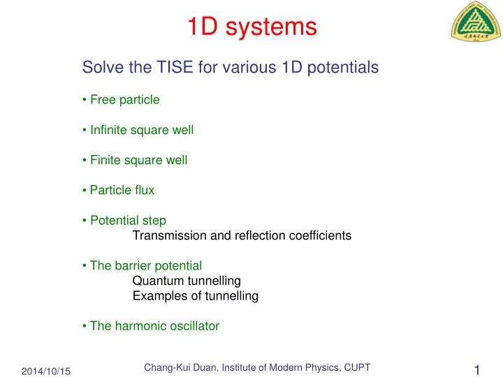
1D systems. Solve the TISE for various 1D potentials Free particle Infinite square well Finite square well Particle flux Potential step Transmission and reflection coefficients The barrier potential Quantum tunnelling Examples of tunnelling The harmonic oscillator.

E N D
1D systems • Solve the TISE for various 1D potentials • Free particle • Infinite square well • Finite square well • Particle flux • Potential step • Transmission and reflection coefficients • The barrier potential • Quantum tunnelling • Examples of tunnelling • The harmonic oscillator
A Free Particle Free particle: no forces so potential energy independent of position (take as zero) Linear ODE with constant coefficients so try Time-independent Schrödinger equation: General solution: Combine with time dependence to get full wave function:
Notes • Plane wave is a solution (just as well, since our plausibility argument for the Schrödinger equation was based on this assumption). • Note signs in exponentials: • Sign of time term (-iωt) is fixed by sign adopted in time-dependent Schrödinger Equation • Sign of position term (±ikx) depends on propagation direction of wave. +ikx propagates towards +∞ while -ikx propagates towards –∞ • There is no restriction on k and hence on the allowed energies. The states form a continuum.
Particle in a constant potential General solutions we will use over and over again Time-independent Schrödinger equation: Case 1: E > V (includes free particle with V = 0 and K = k) Solution: Case 2: E < V (classically particle can not be here) Solution:
V(x) -a a Infinite Square Well Consider a particle confined to a finite length –a<x<a by an infinitely high potential barrier No solution in barrier region (particle would have infinite potential energy). x In the well V = 0 so equation is the same as before General solution: Boundary conditions: Continuity of ψ at x = a: Note discontinuity in dψ/dx allowable, since potential is infinite Continuity of ψ at x = -a:
Infinite Square Well (2) Add and subtract these conditions: Even solution: ψ(x) = ψ(-x) Odd solution: ψ(x) = -ψ(-x) Energy We have discrete states labelled by an integer quantum number
Infinite Square Well (3) Normalization Normalize the solutions Calculate the normalization integral Normalized solutions are
Infinite Square Well (4) Sketch solutions Wavefunctions Probability density 3 1 Note: discontinuity of gradient of ψat edge of well. OK because potential is infinite there.
Infinite Square Well (5) Relation to classical probability distribution Classically particle is equally likely to be anywhere in the box Quantum probability distribution is But so the high energy quantum states are consistent with the classical result when we can’t resolve the rapid oscillations. This is an example of the CORRESPONDENCE PRINCIPLE.
Infinite Square Well (5) – notes • Energy can only have discrete values: there is no continuum of states anymore. The energy is said to be quantized. This is characteristic of bound-state problems in quantum mechanics, where a particle is localized in a finite region of space. • The discrete energy states are associated with an integer quantum number. • Energy of the lowest state (ground state) comes close to bounds set by the Uncertainty Principle: • The stationary state wavefunctions are even or odd under reflection. This is generally true for potentials that are even under reflection. Even solutions are said to have even parity, and odd solutions have odd parity. • Recover classical probability distribution at high energy by spatial averaging. • Warning! Different books differ on definition of well. E.g. • B&M: well extends from x = -a/2 to x = +a/2. Our results can be adapted to this case easily (replace a with a/2). • May also have asymmetric well from x = 0 to x = a. Again can adapt our results here using appropriate transformations.
V(x) I II III V0 x -a a i.e. particle is bound Finite Square Well Now make the potential well more realistic by making the barriers a finite height V0 Region I: Region II: Region III:
Finite Square Well (2) Boundary conditions: match value and derivative of wavefunction at region boundaries: Match ψ: Match dψ/dx: Now have five unknowns (including energy) and five equations (including normalization condition) Solve:
Finite Square Well (3) Even solutions when Cannot be solved algebraically. Solve graphically or on computer Odd solutions when We have changed the notation into q
Finite Square Well (4) Graphical solution k0 = 4 a = 1 Even solutions at intersections of blue and red curves (always at least one) Odd solutions at intersections of blue and green curves
Finite Square Well (5) Sketch solutions Wavefunctions Probability density Note: exponential decay of solutions outside well
Finite Square Well (6): Notes • Tunnelling of particle into “forbidden” region where V0 > E • (particle cannot exist here classically). • Amount of tunnelling depends exponentially on V0 – E. • Number of bound states depends on depth of well, • but there is always at least one (even) state • Potential is even, so wavefunctions must be even or odd • Limit as V0→∞: • We recover the infinite well solutions as we should.
Material A (e.g. AlGaAs) Material B (e.g. GaAs) Electron energy Position Example: the quantum well Quantum well is a “sandwich” made of two different semiconductors in which the energy of the electrons is different, and whose atomic spacings are so similar that they can be grown together without an appreciable density of defects: Now used in many electronic devices (some transistors, diodes, solid-state lasers)
Summary of Infinite and Finite Wells Infinite wellInfinitely many solutions Even parity Odd parity Finite well Finite number of solutions At least one solution (even parity) Evanescent wave outside well. Odd parity solutions Even parity solutions
Particle Flux In order to analyse problems involving scattering of free particles, need to understand normalization of free-particle plane-wave solutions. Conclude that if we try to normalize so that we get A = 0. This problem is related to Uncertainty Principle: Position completely undefined; single particle can be anywhere from -∞ to ∞, so probability of finding it in any finite region is zero Momentum is completely defined Solutions: Normalize in a finite box Use wavepackets (later) Use a flux interpretation
x a b Particle Flux (2) More generally: what is the rate of change of probability that a particle is in some region (say, between x=a and x=b)? Use time-dependent Schrödinger equation:
x a b Particle Flux (3) Flux entering at x=a minus Flux leaving at x=b Interpretation: Note: a wavefunction that is real carries no current
Particle Flux (4) Check: apply to free-particle plane wave. Makes sense: # particles passing x per unit time = # particles per unit length × velocity So plane wave wavefunction describes a “beam” of particles.
Particle flux is nonlinear • Time-independent case: replace • 3D case, • Can use this argument to prove CONSERVATION OF PROBABILITY. • Put a = -∞, b = ∞, then and Particle Flux (5): Notes
V(x) V0 Case 1 0 x > 0, V = V0 Potential Step Consider a potential which rises suddenly at x = 0: x Boundary condition: particles only incident from left Case 1: E > V0 (above step) x < 0, V = 0
Potential Step (2) Continuity of ψ at x = 0: Solve for reflection and transmission amplitudes:
Potential Step (3) Transmission and Reflection Fluxes Calculate transmitted and reflected fluxes x < 0 x > 0 (cf classical case: no reflected flux) Check: conservation of particles
V(x) V0 0 Potential Step (4) Case 2: E < V0(below step) Solution for x < 0same as before Solution for x > 0is now evanescent wave Matching boundary conditions: Transmission and reflection amplitudes: Transmission and reflection fluxes: This time we have total reflected flux.
Some tunnelling of particles into classically forbidden region even for energies below step height (case 2, E < V0). • Tunnelling depth depends on energy difference • But no transmitted particle flux, 100% reflection, like classical case. • Relection probability is not zero for E > V0 (case 1). Only tends to zero in high energy limit, E >> V (correspondence principle again). Potential Step (5): Notes
V(x) I II III V0 0 b Rectangular Potential Barrier Now consider a potential barrier of finite thickness: x Boundary condition: particles only incident from left Region I: Region II: Region III: u = exp(ikx) + B exp(−ikx) u = C exp(Kx) + D exp(−Kx) u = F exp(ikx)
Rectangular Barrier (2) Match value and derivative of wavefunction at boundaries: Match ψ: 1 + B = C + D 1 − B = K/(ik)(C − D) C exp(Kb) + D exp(−Kb) = F exp(ikb) C exp(Kb) − D exp(−Kb) = ik/K F exp(ikb) Match dψ/dx: Eliminate wavefunction in central region:
Rectangular Barrier (3) Transmission and reflection amplitudes: F For very thick or high barrier: |F|2 = Non-zero transmission (“tunnelling”) through classically forbidden barrier region. Exponentially sensitive to height and width of barrier.
V Repulsive Coulomb interaction Incident particles Assume a Boltzmann distribution for the KE, Probability of nuclei having MeV energy is Nuclear separation x Strong nuclear force (attractive) Examples of Tunnelling Tunnelling occurs in many situations in physics and astronomy: 1. Nuclear fusion (in stars and fusion reactors) Fusion (and life) occurs because nuclei tunnel through the barrier
V Distance of α-particle from nucleus Initial α-particle energy Examples of Tunnelling 2. Alpha-decay α-particle must overcome Coulomb repulsion barrier. Tunnelling rate depends sensitively on barrier width and height. Explains enormous range of α-decay rates, e.g. 232Th, t1/2 = 1010 yrs, 218Th, t1/2 = 10-7s. Difference of 24 orders of magnitude comes from factor of 2 change in α-particle energy!
V x Probe Material a Vacuum Examples of Tunnelling 3. Scanning tunnelling microscope A conducting probe with a very sharp tip is brought close to a metal. Electrons tunnel through the empty space to the tip. Tunnelling current is so sensitive to the metal/probe distance (barrier width) that even individual atoms can be mapped. Tunnelling current proportional to and so If a changes by 0.01A (~1/100th of the atomic size) then current changes by a factor of 0.98, i.e. a 2% change, which is detectable STM image of Iodine atoms on platinum. The yellow pocket is a missing Iodine atom
Summary of Flux and Tunnelling The particle flux density is Particles can tunnel through classically forbidden regions. Transmitted flux decreases exponentially with barrier height and width We get transmission and reflection at potential steps. There is reflection even when E > V0. Only recover classical limit for E >> V0 (correspondence principle)
Mass m x V(x) x Simple Harmonic Oscillator Example: particle on a spring, Hooke’s law restoring force with spring constant k: Time-independent Schrödinger equation: Problem: still a linear differential equation but coefficients are not constant. Simplify: change to dimensionless variable
Simple Harmonic Oscillator (2) Asymptotic solution in the limit of very large y: Try it: Equation for H(y):
Simple Harmonic Oscillator (3) Solve this ODE by the power-series method (Frobenius method): Find that series for H(y)must terminate for a normalizable solution Can make this happen after n terms for either even or odd terms in series (but not both) by choosing Hence solutions are either even or odd functions (expected on parity considerations) 0 Label normalizable functions H by the values of n (the quantum number) Hnis known as the nth Hermite polynomial.
is a polynomial of degree Simple Harmonic Oscillator (4) EXAMPLES OF HERMITE POLYNOMIALS AND SHO WAVEFUNCTIONS are normalization constants
Simple Harmonic Oscillator (5) Wavefunctions High n state (n=30) wavefunction Probability density • Decaying wavefunction tunnels into classically forbidden region • Spatial average for high energy wavefunction gives classical result: • another example of the CORRESPONDENCE PRINCIPLE
1) The quantum SHO has discrete energy levels because of the normalization requirement 2) There is ‘zero-point’ energy because of the uncertainty principle. 3) Eigenstates are Hermite polynomials times a Gaussian 4) Eigenstates have definite parity because V(x) = V(-x). They can tunnel into the classically forbidden region. 5) For large n (high energy) the quantum probability distribution tends to the classical result. Example of the correspondence principle. 6)Applies to any SHO, eg: molecular vibrations, vibrations in a solid (phonons), electromagnetic field modes (photons), etc Summary of Harmonic Oscillator
Example of SHOs in Atomic Physics: Bose-Einstein Condensation 87Rb atoms are cooled to nanokelvin temperatures in a harmonic trap. de Broglie waves of atoms overlap and form a giant matter wave known as a BEC. All the atoms go into the ground state of the trap and there is only zero point energy (at T=0). This is a superfluid gas with macroscopic coherence and interference properties. Signature of BEC phase transition: The velocity distribution goes from classical Maxwell-Boltzmann form to the distribution of the quantum mechanical SHO ground state.
H2 molecule V(x) x H H Nuclear separation x SHO levels Example of SHOs: Molecular vibrations VIBRATIONAL SPECTRA OF MOLECULES Useful in chemical analysis and in astronomy (studies of atmospheres of cool stars and interstellar clouds). SHO very useful because any potential is approximately parabolic near a minimum