Download
1 / 52
520 likes | 697 Views
Markov and semi-Markov processes describe the dynamics of biological ion channels. Professor Alan G Hawkes Swansea University. Professor David Colquhoun : Professor of Pharmacology, University College London. Swansea ion-channel team. Alan Hawkes. Assad Jalali. Anton Merlushkin.

E N D
Markov and semi-Markov processes describe the dynamics of biological ion channels Professor Alan G Hawkes Swansea University
Professor David Colquhoun: Professor of Pharmacology, University College London
Swansea ion-channel team Alan Hawkes Assad Jalali Anton Merlushkin
Basic results Bursting behaviour Time Interval Omission (TIO) Joint distributions – maximum likelihood estimation Multiple levels Bursting behaviour with TIO
Channel is modelled as a finite-state Markov process with transition rate matrix Transition probability matrix are eigenvalues of
is a semi-Markov process with kernel density being a matrix whose ijth element is
Is a Markov chain with transition matrix Taking alternate events, the open ones, we have a Markov chain with equilibrium probability vector satisfying The equilibrium distribution of observed open times is
Burst length Gap between bursts Gaps within bursts Total open time per burst Total shut time per burst Number of openings per burst Length of the kth opening in a burst with r openings
Time interval omission (TIO) In this example four actual open intervals make one
Modified kernels Instead of embedding a semi-Markov process at time after an observed interval begins, it is more natural to do so at the start of each such interval. The trouble is that, at such moments, we do not know that the first interval is going to last for at least . The probability that it does last that long, conditional on the starting state is given by vectors for open and closed intervals, respectively. Then the new semi-Markov kernels are given by for open intervals and a similar expression for closed intervals.
Is a Markov chain with transition matrix Taking alternate events, the open ones, we have a Markov chain with equilibrium probability vector satisfying The equilibrium distribution of observed open times is
For define Is the event that no shut period is detected over (0, t) where
Let Theorem. If haseigenvalues Is a polynomial of degree m in t with matrix-valued coefficients Where So, in the interval The exponentials are multiplied by polynomials of degree m.
Asymptotic results We can use the algebra of partitioned matrices to get an alternative Laplace transform expression, which can be also be obtained by the following more appealing direct argument
Theorem: When Q is reversible,detW() = 0 has exactly realroots If Q is irreducible and the roots are distinct, then, as are the right (column) and left (row) where corresponding to eigenvalue eigenvectors of
Applications Joint distributions: it is interesting to study the joint behaviour of neighbouring open/shut pairs of intervals, looking at conditional distributions, means etc. This can be done from the product Likelihood: The likelihood for a whole sequence can found, and maximised to provide parameter estimates from the product Jumps and pulses: The techniques discussed can be used to study the first few events following a jump or a pulse change in agonist concentrations or voltage level, which modify the Q-matrix in known ways.
We have found that a limitation of ML analyses based on records at a single agonist concentration is the statistical correlation between the estimates of the channel opening rate, b, and the shutting rate, a . The correlation coefficient between these estimates is often greater than 0.9, found from the off-diagonals of the Hessian matrix of the likelihood evaluated at its maximum. There is a corresponding diagonal ridge in the likelihood surface. This corresponds to the difficulty in distinguishing between long openings with few interruptions (small a, b ) and many shorter openings separated by very short shuttings (large a , b ) which combine to form a large apparent opening.. However, good estimates can be made if data from recordings at more than one concentration are combined to form an overall likelihood.
Multiple Levels Some channels exhibit more than one conductance level when open. and this raises some complication. The main kernel densities can be found in a manner similar to the two-level case.
The transition rate matrix can then be partitioned in the form We look at an embedded semi-Markov process for which we note the duration of periods of time spent at each level and the “gateway state”, the state in which an occupancy begins. This has a density kernel. where
The difficulty arises because, while we may be sure that the channel has left a particular level for a period in excess of , We may not be sure where it has gone to: it may hop around rapidly between two or more levels before settling on one of them. The trick is to introduce some ‘indeterminacy intervals’ and augment the state space of the semi-Markov process to include states of the form (r, i), which indicates that the channel is in state iat the start of an indeterminacy that follows an observed sojourn at level r.