Download
1 / 28
280 likes | 777 Views
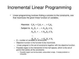
Incremental Linear Programming. Linear programming involves finding a solution to the constraints, one that maximizes the given linear function of variables. D = number of variables or dimensions. Objective function is the function to be maximized.

E N D
Incremental Linear Programming • Linear programming involves finding a solution to the constraints, one that maximizes the given linear function of variables. • D = number of variables or dimensions. • Objective function is the function to be maximized. • Linear program is the set of constraints together with the objective function. • Feasible region is the intersection of the half-spaces, which is the set of points that satisfy all the constraints. • Feasible region can be bounded, unbounded, empty. If empty problem is infeasible Maximize C1X1 + C2X2 + … + CdXd Subject to A1,1X1 + … + A1,dXd ≤ b1 A2,1X1 + … + A2,dXd≤ b2 … An,1X1 + … + An,dXd ≤ bn
Linear Programming • Operations Research has developed many algorithms to solve linear programs that perform well in practice. • Our LP has N linear constants in 2 variables. • Most OR applications have high-dimension (# constraints and variables) and do not work well in low dimensions (# of variables). • Computational Geometry algorithms can do better in low dimensions
Linear Program (H,c) • H is set of n two-dimensional constraints • gives objective function • GOAL: find so that and is maximized • Let C denote feasible region for (H, c)
Linear Program • Four possible cases • Convention: to give unique solution for 3rd example, choose lexicographically smallest point. C p P e Unbounded Return ray EC Infeasible No solution Non-Unique Solution Unique (vertex) solution
Incremental 2-dimensional linear programming • Add constraints one by one • Maintain optimal vertex of intermediate feasible region. • Slight problem, requires that solution exists! • Not true for unbounded linear program • We will use subroutine for this
Unbounded LP (H,c) • If (H,c) unbounded return ray in C • else return so that is bounded. (h1 and h2 are certificates) certificates
Linear Programming • Let (H,c) be bounded linear program • h1 and h2 are certificates returned by UnboundedLP(H,c) • Number remaining halfplanes h3,h4,…,hn Let Ci = feasible region with respect to halfplanes h1-hi = Note: Fact: ci = Ø then cj = Ø for all j≥i (and LP is infeasible)
How does optimal vertex change as we add hi? • Vi is optimal vertex for Ci • Li is line bounding hi
Lemma 4.5 :Let ci and vi be defined as before(i)If vi-1 Îhi, then vi = vi-1 (ii)If vi-1 Ï hi, then either ci = f or viÎ li . Proof :Let vi-1 Î hi (1) ci = ci-1 Ç hi implies ciÍ ci-1 (2) vi-1 Î ci-1 and viÎ hi implies vi-1 Î ci Note that the optimal point in ci cannot be better than optimal point in ci-1 (smaller) implies vi-1 is optimal in ci
Let vi-1 ÏhiSuppose ci ¹f and viÏ li (contradiction) (1) Consider segment vector vi-1 vi -by definition vi-1Îci-1 -since ciÌ ci-1 ,viÎ ci-1 -since ci-1 is convex this implies the vector vi-1viÌ ci-1 (2) since vi-1 is optimal for ci-1 and fc is linear this implies fc(p) increases monotonically along the vector vi1vi as p moves from vi to vi-1.
(Proof continued) (3) Consider intersection point q of vector vi-1vi and li - q exists since vi-1Ïhi and viÎc i Since vector vi-1vi Îci-1 , q must be in ci but value of the objective function increases along the vector vi-1vi so fc(q) > fc(vi) which is a contradiction to the definition of vi
To update optimal point : (1) If vi-1Î hi then we are done (vi = vi-1) (2) If vi-1Ïhi we need to find vi on li but this is just a one dimensional LP One-Dimensional LP : Find p on li that maximizes fc(p) subject to constraints p Î h j , 1£ j £ i. Without loss of generality, assume li is x-axis and let xj = liÇ hj. We will now see how to solve one dimesional LP
To solve One-Dimensional LP : x left = max 1£ j < i {x j | li Ç hj is bounded to left } x right = min 1£ j < i {x j | li Ç hj is bounded to right} The interval [x left, x right] is a feasible region - LP is infeasible if x left > x right - Otherwise, optimal point is x left or x right Running time of One-Dimensional LP : O(n)
Algorithm: Two Dimensional LP(H,c) Input :LP(H,c) Output :Infeasible, Unbounded (and ray in c), or solution point p maximizing fc(p) 1. Run UNBOUNDEDLP(H,c) report if (H,c) is infeasible or unbounded (and ray in c) 2. Let h1 and h2 be certificates returned by UNBOUNDEDLP(H,c) letv2 = h1Ç h2 and let h3,h4, ...,hn be half planes in H for i = 3 to n if vi-1 Î hi then vi := vi-1 else vi := 1DLP({h1, h2, ... , hi-1}, c) if vi doesn’t exist report infeasible. endif end for return vn end algorithm
Running time : • Unbounded LP implies O(n) (We will see later) • - Each iteration O(i) implies å O(i) = O(n2) • Therefore O(n2) in total. • Correctness : • Follows from Lemma 4.5 (each iteration have correct) • But this algorithm is worse than the one for constructing entire convex region.
Incremental LP • Nice and simple. • But…takes O(n2) time in worst case, which is worse than the previous algorithm that computed the entire feasible region!
Is our analysis too crude?i.e. is algorithm actually better than we thought? • Algorithm has n-2 stages, (each time add a half plane) • We said stage i takes O(i) time, the time for 1D-LP with i half-planes. • Note however: stage i takes: • O(i) time if optimal vertex changes do 1D-LP (previous optimal is not in hi). • O(1) time if optimal vertex does not change (previous optimal is in hi, so still optimal).
Question: how many times can optimal vertex change? • Idea: if we can show it changes only say k times, than we can bound running time at O(k•n). • Unfortunately: there are cases in which optimal vertex can change every time…
Question: how many times can optimal vertex change? • Thus, if we consider the planes (in this order), then the optimal vertex changes every time, and we have to do a 1D-LP each time! Running time O(n2) !! • Notice however, that if we had been lucky and added the vertices in the reverse order then the optimum would never change! • Hmm… can we determine the right order in which to add the planes?
Randomization • Unfortunately, we can not really determine the exact best order without a lot of work… • Answer: Randomization Choose a random permutation of the planes and add them in that order. • We could have bad luck and pick a bad order that gives O(n2) running time. • But most orders are not bad (as we’ll see) and so usually we do pretty well.
Changes to Algorithm • Before start adding half-planes, randomly permute them. The running time is O(n). • RandomPermutation(A) input: A[1…n] output: A[1…n] --- permuted randomly for i = n downto 2 random_index = Random(i) swap(A[i], A[random_index]) endfor
Randomized incremental algorithm • Algorithm is now randomized algorithm.random choices made in permutation subroutine • What is running time of randomized incremental algorithm? • Depends on permutation, and there are (n-2)! of them… • We’ll study the expected running time. • Each permutation of input is equally likely and doesn’t depend on the input planes • No assumptions made on input and so expectation is w.r.t. random order in which half-planes are treated and holds for any set of half-planes.
Expected running time • Theorem 4.8: The 2D-LP with n constraints can be solved in O(n) expected time using a randomized incremental algorithm. • Proof: • Running time of RandomPermutation() and UnboundedLP() are O(n). We’ll see the latter one. • Need to consider time for adding n-2 half-planes.
Expected running time • Adding a half-plane takes • Constant time if the optimum doesn’t change • O(i) time if does change (ith half-plane with 1D-LP). • We will bound time for all 1D-LPs. • Let Xi be random variable:
Expected running time • If Xi = 1, then 1D-LP takes O(i) time. Otherwise, adding hi takes O(1) time. Total time adding all half-planes (with 1D-LP) is: • We bound this sum using linearity of expectation: expected value of sum of RV’s is sum of the expected values.
Expected running time • What is E[Xi]? Probability that vi-1 hi. • “Backward analysis” • Algorithm done, vn is optimum vertex and vertex of Cn. • Is it a vertex of Cn-1? The answer is no only if hn is one of half-plane defining vn. How likely is this…? Only at most 2/(n-2).
Expected running time • And in general, to bound E[Xi] we • Fix subset of first i half-planes (determine Ci). • Compute a new optimum when adding hi if hi was one of two half-planes defining new optimum. E[Xi] = 2/(i-2) . • So total bound:
Expected running time Randomized Incremental Algorithm takes O(n) expected time. Important: Expectation is only with respect to random permutation and applies to any input set.