Download
1 / 34
340 likes | 658 Views
Ann Nicholson. Bayesian Networks and Causal Modelling. School of Computer Science and Software Engineering Monash University. Overview. Introduction to Bayesian Networks (BNs) Summary of BN research projects Varieties of Causal intervention

E N D
Ann Nicholson Bayesian Networks and Causal Modelling School of Computer Science and Software Engineering Monash University
Overview • Introduction to Bayesian Networks (BNs) • Summary of BN research projects • Varieties of Causal intervention • PRICAI2004: K. Korb, L. Hope, A. Nicholson, K. Axnick • Learning Causal Structure • CaMML software
Probability theory for representing uncertainty • Assigns a numerical degree of belief between 0 and 1 to facts • e.g. “it will rain today” is T/F. • P(“it will rain today”) = 0.2 prior probability (unconditional) • Posterior probability (conditional) • P(“it wil rain today” | “rain is forecast”) = 0.8 • Bayes’ Rule: P(H|E) = P(E|H) x P(H) P(E)
Bayesian networks • A Bayesian Network (BN) represents a probability distribution graphically (directed acyclic graphs) • Nodes: random variables, • R: “it is raining”, discrete values T/F • T: temperature, cts or discrete variable • C: colour, discrete values {red,blue,green} • Arcs indicate conditional dependencies between variables • P(A,S,T) can be decomposed to P(A)P(S|A)P(T|A)
X Flu P(Flu=T) = 0.05 P(Te=High|Flu=T) = 0.4 P(Te=High|Flu=F) = 0.01 Y Te Q Th P(Th=High|Te=H) = 0.95 P(Th=High|Te=L) = 0.1 Bayesian networks (cont.) • There is a conditional probability distribution (CPD or CPT) associated with each node. • probability of each state given parent states “Jane has the flu” Models causal relationship “Jane has a high temp” Models possible sensor error “Thermometer temp reading”
Flu Flu Flu Flu TB Flu Y Y Te Te Th Th Th BN inference • Evidence: observation of specific state • Task: compute the posterior probabilities for query node(s) given evidence. Te Te Diagnostic inference Predictive inference Mixed inference Intercausal inference
Causal Networks • Arcs follow the direction of causal process • Causal Networks are always BNs • Bayesian Networks aren't always causal
Early BN-related projects • DBNS for discrete monitoring (PhD, 1992) • Approximate BN inference algorithms based on a mutual information measure for relevance (with Nathalie Jitnah, 1996-1999) • Plan recognition: DBNs for predicting users actions and goals in an adventure game (with David Albrecht,Ingrid Zukerman,1997-2000) • DBNs for ambulation monitoring and fall diagnosis (with biomedical engineering, 1996-2000) • Bayesian Poker (with Kevin Korb,1996-2003)
Knowledge Engineering with BNs • Seabreeze prediction: joint project with Bureau of Meteorology • Comparison of existing simple rule, expert elicited BN, and BNs from Tetrad-II and CaMML • ITS for decimal misconceptions • Methodology and tools to support knowledge engineering process • Matilda: visualisation of d-separation • Support for sensitivity analysis • Written a textbook: • Bayesian Artificial Intelligence, Kevin B. Korb and Ann E. Nicholson, Chapman & Hall / CRC, 2004. www.csse.monash.edu.au/bai/book
Current BN-related projects • BNs for Epidemiology (with Kevin Korb, Charles Twardy) • ARC Discovery Grant, 2004 • Looking at Coronary Heart Disease data sets • Learning hybrid networks: cts and discrete variables. • BNs for supporting meteorological forecasting process (DSS’2004) (with Ph. D student Tal Boneh, K. Korb, BoM) • Building domain ontology (in Protege) from expert elicitation • Automatically generating BN fragments • Case studies: Fog, hailstorms, rainfall. • Ecological risk assessment • Goulburn Water, native fish abundance • Sydney Harbour Water Quality
Other projects • Autonomous aircraft monitoring and replanning (withPh.D. studentTim Wilkin,PRICAI2000, IAV2004) • Dynamic non-uniform abstraction for approximate planning with MDPs (with Ph.D. student Jiri Baum)
Flu Flu Observation and Intervention • Inference from observations • Predictive reasoning (finding effects) • Diagnostic reasoning (finding causes) • Inference with interventions • Predictive reasoning • Not diagnostic reasoning • Causal reasoning shouldn't go against causality. Te Te Th Th Diagnostic inference Predictive inference
Pearlian Determinism • Pearl's reasons for determinism: • Determinism is intuitive • Counterfactuals and causal explanation only make sense with a deterministic interpretation • Any indeterministic model can be transformed into a deterministic model • We see no reason for assuming determinism
Defining Intervention I • Arc cutting • More intuitive • Intervention node • Intervention node • More general interventions • Much easier to implement • To simulate arc cutting: P(C| c, Ic)=1 Arc cutting isn’t general enough
Defining Intervention II We define an intervention on model M as: • M augmented with Ic (M') where: • Ic has the purpose of manipulating C • Ic is exogenous (has no parents) in M' • Ic directly causes (is a parent of) C • To preserve the original network: PM'(C| c,¬ Ic) = PM' (C| c) where c are the original parents of C. We also define P*(C) as the intended distribution.
Varieties of Intervention: Dependency The degree of dependency of the effect upon existing parents. • An independent intervention cuts the child off from its other parents. Thus, PM'(C| c, Ic) = P*(C) • A dependent intervention allows any parent interaction.
Varieties of Intervention : Indeterminism The degree of indeterminism of the effect. • A deterministic intervention sets the child to one particular state. • A stochastic intervention sets the child to a positive distribution. Dependency and Determinism • characterize any intervention • Pearlian interventions are independent and deterministic
Varieties of Intervention : Effectiveness We've found the idea of effectiveness useful. If P*(C) is what's intended and r is the effectiveness, then PM'(C | c, Ic) = r × P*(C) + (1-r) × PM'(C | c) This is a dependent intervention.
Summary of Causal Intervention • A taxonomy of intervention types • More realistic interventions (e.g., partial effectiveness) • A GUI which handles some varieties of intervention • Pearlian • Partially effective • Extensible to deal with other types of interaction explicitly
Learning Causal Structure • This is the real problem; parameterizing models is relatively straightforward estimation problem. • Size of the dag space is superexponential: • Number of possible orderings: n! • Times number of possible arcs: Cn2 • Minus number of possible cyclic graphs • More exactly (Robinson, 1977): f(n) = (-1)i+1 Cni 2i(n-i)f(n-i) so for • n=3, f(n)=25 • n=5, f(n)=25,000 • n=10, f(n) 4.2x10¹⁸
Learning Causal Structure • There are two basic methods: • Learning from conditional independencies (CI learning) • Learning using a scoring metric (Metric learning) • CI learning (Verma and Pearl, 1991) • Suppose you have an Oracle who can answer yes or no to any question of the type: is X conditional independence Y given S? • Then you can learn the correct causal model, up to statistical equivalence (patterns).
Statistical Equivalence • Two causal models H1 and H2 are statistically equivalent iff they contain the same variables and joint samples over them provide no statistical grounds for preferring one over the other. • Examples • All fully connected models are equivalent. • A B C and A B C. • A B D C and A B D C.
Statistical Equivalence (cont.) • (Verma and Pearl, 1991): Any two causal models over the same variables which have the same skeleton (undirected arcs) and the same directed v-structures are statistically equivalent. • Chickering (1995): If H1 and H2 are statistically equivalent, then they have the same maximum likelihoods relative to any joint samples max P(e|H1,1) = max P(e|H2,2) where i is a parameterization of Hi
Other approaches to structure learning • TETRAD II: Spirtes, Glymour and Scheines (1993). Implemented in their PC algorithm • Doesn't handle well with weak links and small samples (demonstrated empirically in Dai, Korb, Wallace & Wu (1997)). • Bayesian LBN: Cooper & Herskovits' K2 (1991, 1992) • Compute P(hi|e) by brute force, under the various assumptions which reduce the computation of PCH(h,e) to a polynomial time counting problem. • But the hypothesis space is exponential; they go for dramatic simplification by assuming we know the temporal ordering of the variables.
Learning Variable Order • Reliance upon a given variable order is a major drawback to K2 • And many other algorithms (Buntine 1991, Bouckert 1994, Suzuki 1996, Madigan & Raftery 1994) • What's wrong with that? • We want autonomous AI (data mining). If experts can order the variables they can likely supply models. • Determining variable ordering is half the problem. If we know A comes before B, the only remaining issue is whether there is a link between the two. • The number of orderings consistent with dags is exponential (Brightwell & Winkler 1990; number complete). So iterating over all possible orderings will not scale up.
Statistical Equivalence Learners • Heckerman & Geiger (1995) advocate learning only up to statistical equivalence classes (a la TETRAD II). • Since observational data cannot distinguish btw equivalent models, there's no point trying to go further. Madigan, Andersson, Perlman & Volinsky (1996) follow this advice, use uniform prior over equivalence classes. Geiger and Heckerman (1994) define Bayesian metrics for linear and discrete equivalence classes of models (BGe and BDe)
Statistical Equivalence Learners Wallace & Korb (1999): This is not right! • These are causal models; they are distinguishable on experimental data. • Failure to collect some data is no reason to change prior probabilities. E.g., If your thermometer topped out at 35C, you wouldn't treat 35C and 34C as equally likely. • Not all equivalence classes are created equal: { A B C, A B C, A B C } { A B C } • Within classes some dags should have greater priors than others… E.g., • LightsOn InOffice LoggedOn v. • LightsOn InOffice LoggedOn
Full Causal Learners So… a full causal learner is an algorithm that: • Learns causal connectedness. • Learns v-structures. Hence, learns equivalence classes. • Learns full variable order. Hence, learns full causal structure (order + connectedness). • TETRAD II: 1, 2. • Madigan et al.; Heckerman & Geiger (BGe, BDe): 1, 2. • Cooper & Herskovits' K2: 1. • Lam and Bacchus MDL: 1, 2 (partial), 3 (partial). • Wallace, Neil, Korb MML: 1, 2, 3.
CaMML • Minimum Message Length (Wallace \& Boulton 1968) uses Shannon's measure of information: I(m) = - log P(m) • Applied in reverse, we can compute P(h,e) from I(h,e). • Given an efficient joint encoding method for the hypothesis & evidence space (i.e., satisfying Shannon's law), MML: Searches {hi} for that hypothesis h that minimizes I(h) + I(e|h). • Applies a trade-off between • Model simplicity • Data fit Equivalent to that h that maximizes P(h)P(e|h) --- i.e., P(h|e).
MML search algorithms MML metrics need to be combined with search. This has been done three ways: • Wallace, Korb, Dai (1996): greedy search (linear). • Brute force computation of linear extensions (small models only) • Neil and Korb (1999): genetic algorithms (linear). • Asymptotic estimator of linear extensions • GA chromosomes = causal models • Genetic operators manipulate them • Selection pressure is based on MML • Wallace and Korb (1999): MML sampling (linear, discrete). • Stochastic sampling through space of totally ordered causal models • No counting of linear extensions required
Empirical Results • A weakness in this area --- and AI generally. • Papers based upon very small models, loose comparisons. • ALARM often used --- everything gets it to within 1 or 2 arcs. • Neil and Korb (1999) compared CaMML and BGe (Heckerman & Geiger's Bayesian metric over equivalence classes), using identical GA search over linear models: • On KL distance and topological distance from the true model, CaMML and BGe performed nearly the same. • On test prediction accuracy on strict effect nodes (those with no children), CaMML clearly outperformed BGe.
Extensions to original CaMML • Allow specification of prior on arc • O’Donnell, Korb, Nicholson • Useful for combining expert and automated methods • Learning local structure • Logit models (Neill, Wallace, Korb) • Hybrid networks - CPT or decision trees (O’Donnell, Allison, Korb, Hope) (Uses MCMC search)
CaMML • Information and executables available at www.datamining.monash.edu.au/software/camml • Linear and Discrete versions • Weka wrapper available