Download
1 / 65
670 likes | 1.31k Views
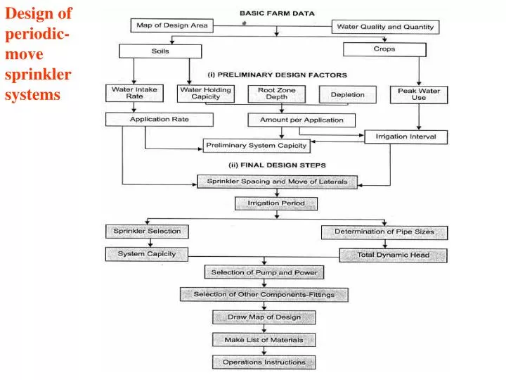
Design of periodic-move sprinkler systems. Design of continuous -move sprinkler systems. Available moisture for different major soil categories. Available moisture for different major soil categories. Ranges of maximum effective rooting depth (z r ) for common crops (Source: FAO,1998).

E N D
Ranges of maximum effective rooting depth (zr) for common crops (Source: FAO,1998)
Ranges of maximum effective rooting depth (zr) for common crops (Source: FAO,1998)
Ranges of maximum effective rooting depth (zr) for common crops (Source: FAO,1998)
Equation 1 dnet = (FC – PMP) * RZD * P dnet = readily available moisture or met depth of water application per irrigation for the selected crop (mm) FC = soil moisture at field capacity (mm/m) PWP = soil moisture at the permanent wilting point (mm/m) RZD = the depth of soil that the roots exploit effectively (m) P = the allowable portion of available moisture permitted of depletion by the crop before the next irrigation
Equation 2 Volume of water to be applied (m3) = 10*A*d A = area proposed for irrigation (ha) d = depth of water application (mm)
Example 1 The following soil and crop data are provided: Area to be irrigated = 18 ha Soil: medium texture, loam Crop: Wheat with peak daily water use = 5.8 mm/day Available moisture (FC – PWP) = 140 mm/m P = 50% or 0.5 RZD = 0.7 m Soil infiltration rate = 5 – 6 mm/hr Average wind velocity in September = 10 km/hr Average wind velocity in October = 11 km/hr
dnet = 140 * 0.7 * 0.5 = 49 For an area of 18 ha, using Equation 2, a net application of 8820 m3(10*18*49) of water will be required per irrigation to bring the root zone depth of the soil from the 50% allowable depletion level to the field capacity
Irrigation frequency at peak demand and irrigation cycle Equation 3 Irrigation frequency (IF) = dnet/wu IF = irrigation frequency (days) dnet = net depth of water application (mm) Wu = peak daily water use (mm/day)
Example 2 Irrigation Frequency (IF) = 49m/5.8mm/day = 8.4 days The system should be designed to provide 49 mm every 8.4 days. For practical purpose, fractions of days are not used for irrigation frequency purpose. Hence the irrigation frequency should be 8 days, with a corresponding dnet of 46.4 mm (5.8 * 8) and a moisture depletion of 0.47 (46.4/(140*0.7))
Gross depth of water application Equation 4 dgross = dnet/E E = the farm (or unit) irrigation efficiency.
Farm irrigation efficiencies for sprinkler irrigation in different climates (Source: FAO,1982)
Example 3 Assuming a moderate climate for the area under consideration and applying Equation 4, the gross depth of irrigation should be: dgross = 46.4/0.75 = 61.87 mm
Preliminary system capacity Equation 5 Q = 10*A*dgross/I*Ns*T Q = system capacity (m3/hr) A = design area (ha) d = gross depth of water application (mm) I = irrigation cycle (days) Ns = number of shifts per day T = irrigation time per shift (hr)
Example 4 The area to be irrigated is 18 ha. In order to achieve the maximum degree of equipment utilization, it is desirable, but not always necessary, that the irrigation system should operate for 11 hours per shift at 2 shifts per day during peak demand and take an irrigation cycle of 7 days to complete irrigating the 18 ha. Q = 10*18*61.87 / 7*2*11 = 72.3 m3/hr
Effect of pressure on water distribution pattern of a two nozzle sprinkler When the sprinkler operates at too low pressure, the droplet size is large. The water would then concentrate in a form of a ring at the distance from the sprinkler. This is very clear with the single nozzle sprinkler, giving a distribution resembling a doughnut
When the pressure is too high, the water breaks into very fine droplets, settling around the sprinkler in no wind conditions. Under the wind conditions, the distribution pattern is easily distorted
Nozzle size indicate the diameter of the orifice of the nozzle. Pressure is the sprinkler operating pressure at the nozzle. Discharge indicates the volume of water per unit time that the nozzle provides at a given pressure Wetted diameter shows the diameter of the circular area wetted by the sprinkler when operating at a given pressure and no wind The sprinkler spacing shows the pattern in which the sprinklers are laid onto the irrigated area. A 12m*18m spacing means that sprinklers are spaced at 12 m along the sprinkler lateral line and 18m between sprinkler lines.
Maximum sprinkler spacing as related to wind velocity, rectangular pattern
Maximum sprinkler spacing as related to wind velocity, square pattern
Maximum precipitation rates to use on level ground * Rates increase with adequate cover and decrease with land slope and time
Suggested maximum sprinkler application rates for average soil, slope, and tilth(Source: Keller and Bliesner)
Equation 6 Ts = dgross/Pr Ts = set time (hr) Pr = sprinkler precipitation rate (mm/hr) Ts = 61.97/5.16 = 11.99 hours
Equation 7 Q = Nc * Ns * Qs Q = system capacity (m3/hr) Nc = the number of laterals operating per shift Ns = the number of sprinklers per lateral Qs = the sprinkler discharge (from the menu factories tables) Q = 4 * 20 * 1.16 = 92.8 m3/hr.
When preparing the layout of the system one should adhere to two principles, which are important for the uniformity of water application. For the rectangular spacing the laterals should be placed across the prevailing wind direction. Where possible, laterals should run perpendicular to the predominant slope in order to achieve fairly uniform head lost.
System layout based on a 12m*18 m spacing and short laterals
Chirstiansens “F” factors for various numbers of outlets (Source: Keller and Bliesner, 1990)
Q = The discharge or flow rate within that section of the pipe, the units depending on the chart being used (m3/hr). L= The length of pipe for that section (m) D = The pipe size diameter (mm). HL= The friction loss of the pipe (m).
Example 5 Where the mainline is located at the middle of the field, the maximum length of the lateral is 150 meters. It will have 13 sprinklers operating at the same time, delivering 1.16 m3/hr each at 350 kPa pressure. The flow at the beginning of the lateral will be: Q = 13 * 1.16 = 15.08 m3/hr The friction loss for a discharge of 15.08 m3/hr will be: HL = 0.013 * 150 = 1.95 m
By taking into consideration the “F” factor corresponding to 13 outlets (sprinklers): HL = 0.013 * 150 *0.373 = 0.73 If instead of 76 mm, 63 mm pipe is used then: HL = 0.033 * 150 *0.373 = 1.85m The friction losses for the 18 m aluminium pipe (header) with flow of 15.08 m3/hr: HL = 0.013 * 18 = 0.23 m for the 76 mm pipe. HL = 0.033 * 18 = 0.59 m for the 63 mm pipe.
The total friction losses in the 76 mm lateral, when the header is used, are 0.96 m (0.73+0.23). The total friction losses in the 63 mm lateral, when the header is used, are 2.44 m (1.85+0.59).
Asbestos-cement pipe classes and corresponding pressure rating
System layout and pipe sizing based on a 12m*18 m spacing and short laterals (first attempt at pipe sizing)
Example 6 Position 1 Difference in elevation = 3.5 meters (108-104.5) Sprinkler operating pressure = 35 meters 20% allowable pressure variation = 0.2 *35 = 7 meters Lateral friction losses = 0.96 meters The total of 46.46 (3.5 +35 +7+0.96) meters, exceeds the pressure rating of class 4 uPVC pipe, which is 40 meters, obliging the use of the next class of pipe, which is class 6.