Download
1 / 41
410 likes | 552 Views
Have We Reached the Limit of Weather Predictability?. J. Shukla George Mason University (GMU) Center for Ocean-Land-Atmosphere Studies (COLA) with contributions from: D. Straus, T. DelSole, J. Kinter Lorenz Symposium American Meteorological Society Annual Meeting, San Diego, CA 13 January 2005.

E N D
Have We Reached the Limit of Weather Predictability? J. ShuklaGeorge Mason University (GMU)Center for Ocean-Land-Atmosphere Studies (COLA)with contributions from:D. Straus, T. DelSole, J. Kinter Lorenz SymposiumAmerican Meteorological Society Annual Meeting, San Diego, CA 13 January 2005
Outline • Introduction (Tellus, 1965; Lorenz: Tellus, 1969; Tellus, 1982) • The “Knife’s Edge”: -5/3 and -3 energy spectra (observations) • ECMWF Forecast Skill, 1982-2002: Revisiting Lorenz (1982) • Predictability of Space-Time Averages • The Future: Conjectures and Suggestions
Lorenz, E. N., 1965: A Study of the Predictability of a 28-Variable Model Tellus, 17, 321-333 Dynamics of Error Growth Variability: Dependence on the State of the Flow 28 – Variable QG 2-level model whose weather is chaotic • First Recognition of the variability of error growth, and of the role of current flow structure • Perhaps first to calculate the fastest growing initial perturbation (which were later identified as singular vectors) • Nearly complete treatment of short-range predictability (error growth) problem
Lorenz, E. N., 1969: The Predictability of a Flow Which Contains Many Scales of Motion. Tellus, 21, 289-307 Dynamics of Average Error Growth: Dependence on the Equilibrium Spectrum • First Recognition of the Role of the Equilibrium Atmospheric Spectrum • Emphasis on Scale-Dependence of Error and Error Growth • Role of simple Advective Non-Linearity in controlling Error Growth
A Fundamental Question in Weather Predictability A Dynamical System is : TYPE 1 – characterized by an infinite range of predictability TYPE 2 – the range of predictability is finite, but can be increased indefinitely by decreasing the size of the initial error TYPE 3 – the range of predictability is finite and intrinsically limited Does the Weather Constitute a Type 2 or a Type 3 System?
System of Equations Simplest System – barotropic flow on an f-plane Isotropic and Homogeneous (turbulent-like) Consistent Quasi-Normal (QN) Closure for errors: Error Growth is linearized until errors reach saturation QN Closure is consistent with linearization Lorenz has been incorrectly criticized for this!
Top curve is energy spectrum (E / l)1/4 Error Propagates upscale Error at 1 day Error at 5 hrs l 1/4 = (2 p / k) 1/4 (l = wavelength)
The Growth of Very Small Errors • Basic Idea – Reduce the Size of the Initial Error by putting it on smaller and smaller scales • Ultimate Predictability controlled bythe predictability time T= time necessary for the error to propagate “upscale” from very, very small initial scale to a finite, pre-chosen scale • How does T behave as the initial error gets infinitely small? This tells us if we haveTYPE 2 orTYPE 3 behavior! • For a Spectrum E(k) ~ k -3 or steeper: • T becomes infinite (thus TYPE 2) • For a Spectrum E(k) less steep than k -3: • T is finite (thus TYPE 3)
The Knife’s Edge “…if the energy per unit wave number obeys aminus-three or higher negative power law, … the series for [the range of predictability] would fail to converge.” -Lorenz, 1969: The predictability of a flow which possesses many scales of motion. Tellus, pg. 304.
Eddy Circulation Time • T(k) = L/U = k-1 (kE)-1 = (E k3 )-1/2 • Tennekes and Lumley 1972; Lilly 1973 • If E(k) = k-b, then T(k) = k(b-3)/2 • For b > 3, time scale increases with k the sum of T(k) does not converge. • Range of Predictability “can be increased indefinitely by reducing the observational errors.” • For b < 3 (e.g., k-5/3), time scale decreases with k the sum of T(k) converges. • Range of Predictability “cannot be lengthened by bettering observations.”
The “Knife’s Edge” – The Observed Spectrum -3 spectrum -5/3 spectrum synoptic scales mesoscales
Does the Observed -5/3 Spectrum Imply that the Range of Predictability Cannot be Lengthened by Reducing Initial Error? • Perhaps the eddies associated with the observed -5/3 spectrum do not interact with the large scale
Decoupling of Rotational and Divergent Waves in Resonant Triads • f-plane Greenspan, 1969 • -plane Longuet-Higgins and Gill, 1967 • Stratified flow Phillips 1968; Lelong and Riley 1991 • Rotating stratified flow Bartello 1995; Embid and Majda 1998 • Rotating shallow-water flow Warn 1986; Embid and Majda 1996
High Resolution Simulations from UKMO and SkyHi Koshyk and Hamilton, 2001, J. Atmos. Sci., 335
Recent Developments: k-5/3 Spectrum May Be Purely QG Tung and Orlando, 2003: J Atmos. Sci
Is k-5/3 an Artifact of Insufficient Dissipation and/or Resolution? K. Shafer Smith, 2004, J. Atmos. Sci., 937–942. Simulated k-5/3 disappears with higher resolution or stronger hyperviscosity Case B (upper dashed): Reproduces Tung & Orlando
Nastrom and Gage, 1985: A climatology of atmospheric wavenumber spectra of wind and temperature observed by commercial aircraft. J. Atmos. Sci., 42, 950–960.
Commentary • The question remains open whether the observed -5/3 spectrum and the underlying arguments are relevant for predictability of the real atmosphere • The nature of mesoscales is dominated by moisture-driven circulation and gravity waves • The energy propagation in the mesoscales (from observations) is from the large to the small scales, not the other way around • In fact, despite 40 years of research, we still cannot definitively state whether the range of predictability cannot be increased indefinitely
Lorenz, E. N., 1982: Atmospheric Predictability Experiments with a Large Numerical Model. Tellus, 34, 505-513 • Estimates of the lower and upper bounds of predictability of instantaneous weather patterns for ECMWF forecast system • Lower bound: skill of “current” operational forecasting procedures • Upper bound: Growth of initial error, defined as the difference between two forecasts valid at the same time (Lorenz curves) “Additional improvements at extended range may be realized if the one-day forecast is capable of being improved significantly.”
ECMWF 500 hPa Error Evolution 1981 – 2002 N.Hem & S.Hem D+1 Forecast error Intrinsic Error Doubling Time A. Hollingsworth ECMWF - Sloan Conference on Weather Predictability 2003
Evolution of 1-Day Forecast Error, Lorenz Error Growth, and Forecast Skill for ECMWF Model(500 hPa NH Winter)
The Known, The Unknown and The Unknowable in Predictability of WeatherSavannah, Georgia, Feb 17-19, 2003(Organizers: D. Straus, B. Kirtman, J. Shukla) Jesse Ausubel Erik Lindborg Peter Bartello Ed Lorenz Lennart Bengtsson* Franco Molteni* Tim DelSole Tim Palmer Kerry Emanuel Richard Peltier Ross Hoffman Kamal Puri Tony Hollingsworth Ed Schneider Rene Laprise Zoltan Toth* Doug Lilly Geoff Vallis
Interim Summary • In spite of the k -5/3 spectrum, • operational forecasts show that as the resolution is increased, the range of predictability increases even though the initial error growth rates increase! • The progress NWP has already made in the past 30 years clearly suggests that, with higher resolution models and improved physical parameterizations and data assimilation techniques, the initial error can be further reduced, and the range of predictability further lengthened.
Predictability of Space- and Time-Averages: Influence of the Boundary Conditions INFLUENCE OF OCEAN ON ATMOSPHERE • Tropical Pacific SST • Arabian Sea SST • North Pacific SST • Tropical Atlantic SST • North Atlantic SST • Sea Ice • Global SST (MIPs) INFLUENCE OF LAND ON ATMOSPHERE • Mountain / No-Mountain • Forest / No-Forest (Deforestation) • Surface Albedo (Desertification) • Soil Wetness • Surface Roughness • Vegetation • Snow Cover
Rainfall 1982-83 1988-89 Zonal Wind 1982-83 The atmosphere is so strongly forced by the underlying ocean that integrations with fairly large differences in the atmospheric initial conditions converge, when forced by the same SST (Shukla, 1982). 1988-89
When tropical forcing is very strong, it can enhance even the predictability of extratropical seasonal mean circulation, which, in the absence of anomalous SST, has no predictability beyond weather. Observed SST JFM83 Observed SST JFM89 IC: 12/89 IC: 12/89 Observed SST JFM89 Observed SST JFM83 IC: 12/83 IC: 12/83
Evolution of Climate Models 1980-2000 Model-simulated and observed 500 hPa height anomaly (m) 1983 minus 1989
Vintage 2000 AGCM
Current Limit of Predictability of ENSO (Nino3.4) Potential Limit of Predictability of ENSO 20 Years: 1980-1999 4 Times per Year: Jan., Apr., Jul., Oct. 6 Member Ensembles Kirtman, 2003
Concluding Remarks • The largest obstacles in realizing the potential predictability of weather and climate are inaccurate models and insufficient observations, rather than an intrinsic limit of predictability. • In the last 30 years, most improvements in weather forecast skill have arisen due to improvements in models and assimilation techniques
Improvement in medium-range forecast skill 12-month running mean of anomaly correlation (%) of 500hPa height forecasts
Concluding Remarks • The largest obstacles in realizing the potential predictability of weather and climate are inaccurate models and insufficient observations, rather than an intrinsic limit of predictability. • In the last 30 years, most improvements in weather forecast skill have arisen due to improvements in models and assimilation techniques • The next big challenge is to build a hypothetical “perfect” model which can replicate the statistical properties of past observed climate (means, variances, covariances and patterns of covariability), and use this model to estimate the limits of weather and climate predictability • The model must represent ALL relevant phenomena, including ocean, atmosphere, and land surface processes and the interactions among them
Coupled Ocean-Land-Atmosphere Model Weather Prediction Model of ~2020 ~1 km x ~1 km 100 levels Unstructured, adaptive grids Landscape-resolving (~100 m) ~1 km x ~1 km 50 levels Unstructured, adaptive grids Assumption: Computing power enhancement by a factor of 103-104
THANK YOU! ANY QUESTIONS?